
Introduction to Recommender System and Implementation Using LightFM
Section 1: Introduction to Recommender System
In this blog, I will introduce what is recommender system and why we need it. Recommender system methods are divided into different types, such as content-based filtering, collaborative filtering, and hybrid method. I will first compare the difference between content-based filtering and collaborative filtering, and then give an example of using LightFM to create your own recommender engine.
What does the recommender system do?
In the past few decades, with the rise of Youtube, Amazon, Netflix, and many other such web services, recommendation systems have become more and more important in our lives. From e-commerce (recommendations to interested buyers to products) to online advertising (recommending the right content for the user’s preferences), today’s recommendation system is inevitable in our daily online travel. Generally, a recommendation system is an algorithm designed to recommend related items to users (depending on the industry, these items include watching movies, reading text, buying products, or other algorithms).

Content Based Filtering vs Collaborative Filtering
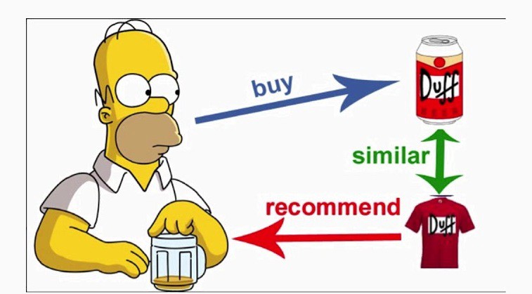
The content-based filtering (CBF) approach uses other information about the user and/or item. Let’s take the classic movie recommendation as an example, the additional information can be, for example, age, gender, job, or any other personal information of the user, as well as category, main actors, duration or other characteristics. It uses similarities in products, services, or content features, as well as information accumulated about the user to make recommendations.
Collaborative filtering (CF) methods for recommender systems are methods that are based solely on the past interactions recorded between users and items in order to produce new recommendations. These interactions are stored in the so-called `user-item interactions matrix’.
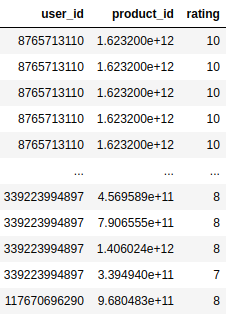
Above shows the sparse user-item interaction matrix, each row contains a user id, item id, and correspoding rates. A dense user-item interactions matrix can be transformed by pivoting the sparse one. In the real world, users can rate implicitly or explicitly. Explicit feedback is raings that users give to the movie they saw, the feedback the users commented to the product they purchased. However, sometimes we may not have the explicit rating. The implicity feedback is obtained from the user activity, such as they clicked an article or a product, played songs, purchased or assigned tags.
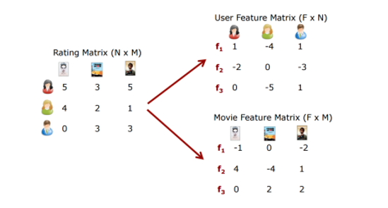
Matrix factorization is a class of collaborative filtering algorithms used in recommender systems. Matrix factorization algorithms work by decomposing the user-item interaction matrix into the product of two lower dimensionality rectangular matrices. For example, the user-item interaction matrix are decomposed into a latent factor of user and a latent factor of item.
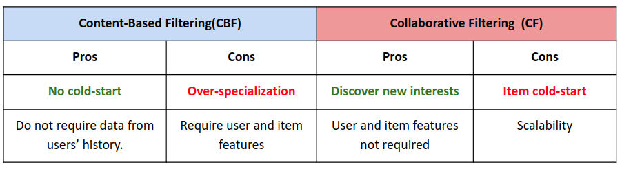
There are both pros and cons for CBF and CF methods. CBF can only recommend the items that within a user’s routine, cannot bring something out of the user’s current interest. CF can figure out what you might like based on finding the other users that close to your interaction history. However, one big problem that CF has is the item/user cold start. When a new product go online and there is no adequate ratings on this new product, it can be hard for the model to recommend this new product to users. Compared with CF, CBF suffers far less from the cold start problem.
What does LightFM propose?
LightFM paper is a hybrid matrix factorisation model representing users and items as linear combinations of their content features’ latent factors. The model outperforms both collaborative and content-based models in cold-start or sparse interaction data scenarios (using both user and item metadata), and performs at least as well as a pure collaborative matrix factorisation model where interaction data is abundant.
In LightFM, like in a collaborative filtering model, users and items are represented as latent vectors (embeddings). However, just as in a CB model, these are entirely defined by functions (in this case, linear combinations) of embeddings of the content features that describe each product or user.
For example, if the movie ‘Wizard of Oz’ is described by the following features: ‘musical fantasy’, ‘Judy Garland’, and ‘Wizard of Oz’, then its latent representation will be given by the sum of these features’ latent representations. In doing so, LightFM unites the advantages of contentbased and collaborative recommenders.
LightFM model learns embeddings (latent representations in a high-dimensional space) for users and items in a way that encodes user preferences over items. When multiplied together, these representations produce scores for every item for a given user; items scored highly are more likely to be interesting to the user.
The user and item representations are expressed in terms of representations of their features: an embedding is estimated for every feature, and these features are then summed together to arrive at representations for users and items.
Section 2: Implement recommendation engines with LightFM
In this section, we will use the LightFM APIs to build up a recommendation engines, starting from preparing and spliting the dataset to evaluating pure CF model and hybrid model.
Step 1: know our data
We have two csv files, one is rating.csv which is the sparse user-item interaction matrix. Another file is features.csv, which contains the features of the item. In this blog, we will not focus on the feature engineering or feature selection part, but on the modeling.
rate.user_id.nunique(), rate.product_id.nunique()
(16838, 3913)
In this dataset, there are 16838 users and 3913 items. To investigate how many ratings each user made, we can use the value_counts() function. To obtain the distribution such as mean, std, quartiles, simply use describe().
rate.user_id.value_counts().describe()

count    16838.000000
mean         5.542760
std          9.645485
min          1.000000
25%          1.000000
50%          3.000000
75%          6.000000
max        240.000000
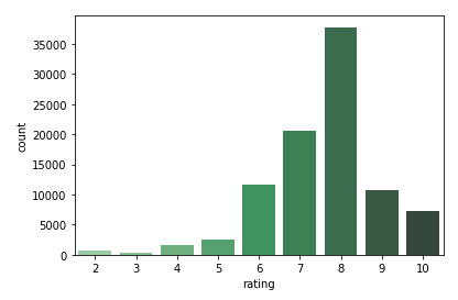
The rating distribution can be visualized by seaborn’s countplot.
sns.countplot(x = 'rating', data = rate, palette = 'Greens_d')
Let’s check what are the item features.
features.iloc[:,:12].head()
| product_id | product_class_id | product_year | product_name | country_name | feature1 | feature2 | feature3 | feature4 | feature5 | num_ratings | avg_ratings | |
|---|---|---|---|---|---|---|---|---|---|---|---|---|
| 0 | 724939662765 | 10084382031 | 10366272 | 1 | 10000.0 | 11480.168232 | 18508.557202 | 11210.750328 | 13386.629203 | 0.0 | 89979024 | 7.4 |
| 1 | 1347498441408 | 3287810067 | 9543813 | 2 | 10001.0 | 21150.199920 | 12395.008618 | 6815.636914 | 0.000000 | 0.0 | 9592056 | 7.6 |
| 2 | 1022923631932 | 28349197767 | 12967668 | 3 | 10002.0 | 19865.256912 | 10852.594147 | 4928.222765 | 0.000000 | 0.0 | 830808 | 7.6 |
| 3 | 5182824340 | 9062972469 | 92275236 | 4 | 10003.0 | 18501.937258 | 20850.229920 | 7673.151638 | 19155.065150 | 0.0 | 8979440 | 7.0 |
| 4 | 956452733050 | 21064890288 | 12967668 | 5 | 10002.0 | 0.000000 | 0.000000 | 0.000000 | 0.000000 | 0.0 | 134272 | 7.6 |
features.iloc[:,12:25].head()
| region_name | food1 | food2 | food3 | food4 | food5 | food6 | food7 | note1 | note2 | note3 | note4 | note5 | |
|---|---|---|---|---|---|---|---|---|---|---|---|---|---|
| 0 | 15000.0 | 1 | 1 | 0 | 0 | 0 | 0 | 1 | 66009.78262062 | 2129.347826598 | 8517.391302474 | 53233.69564536 | 4258.695653196 |
| 1 | 15001.0 | 0 | 0 | 0 | 0 | 0 | 0 | 0 | 3957.57575718 | 122684.84847258 | 3957.57575718 | 67278.78787206 | 3957.57575718 |
| 2 | 15002.0 | 0 | 0 | 0 | 0 | 0 | 1 | 0 | 0 | 180830.7692157 | 0 | 60276.92305884 | 0 |
| 3 | 15003.0 | 1 | 0 | 1 | 0 | 0 | 1 | 0 | 55971.42858822 | 9328.571428758 | 9328.571428758 | 27985.714286274 | 0 |
| 4 | 15004.0 | 0 | 0 | 0 | 0 | 0 | 0 | 0 | 0 | 0 | 0 | 97950 | 0 |
features.iloc[:,25:].head()
| note6 | note7 | note8 | note9 | note10 | note11 | note12 | note13 | class_name | price | |
|---|---|---|---|---|---|---|---|---|---|---|
| 0 | 21293.478262062 | 2129.347826598 | 112855.43479794 | 95820.65217732 | 12776.08695567 | 0 | 0 | 12776.08695567 | 20000 | 19.95 |
| 1 | 3957.57575718 | 7915.15151436 | 7915.15151436 | 3957.57575718 | 3957.57575718 | 91024.24241514 | 23745.454546998 | 47490.90908616 | 20001 | 17.95 |
| 2 | 0 | 0 | 0 | 0 | 30138.461537256 | 60276.92305884 | 30138.461537256 | 30138.461537256 | 20002 | 14.95 |
| 3 | 4664.28571242 | 4664.28571242 | 149257.1428758 | 79292.85715032 | 46642.8571242 | 0 | 0 | 4664.28571242 | 20003 | 12.00 |
| 4 | 97950 | 0 | 0 | 0 | 0 | 97950 | 97950 | 0 | 20004 | 17.20 |
Step2: prepare the dataset for LightFM models
split into train and test set
With the sparse user-item interaction matrix, we first will need to split the dataset into training and testing set. I wrote the function, which can split the sparse interaction matrix by ratio, with the default 0.8. Shuffle is the boolean variable, by default it will shuffle the rows of the dataframe. The function will support encoding the user_id and product_id, as this is the necessary step preparing the dataset. Strings are not allowed, but only integers.
def create_rate_matrix(df, shuffle = True, split_ratio = 0.8):
    '''
    Split the Pandas DataFrame into train and test according to the split_ratio.
    INPUT:
      - df: Pandas DataFrame of interaction data, including user id, product id, and rate.
      - shuffle: boolean, whether to randomly shuffle the dataframe before splitting
      - split_ratio: the ratio of train and test
    OUTPUT:
      - rate_matrix: a dictionary, keys ['train', 'test'], value is coo_matrix of the same shape
    '''
    if shuffle:
        df = df.sample(frac = 1).reset_index(drop = True)
    split_point = np.int(np.round(df.shape[0] * split_ratio))
    df_train = df.iloc[0:split_point]
    df_test = df.iloc[split_point::]
    df_test = df_test[(df_test['user_id'].isin(df_train['user_id']))&\
                     (df_test['product_id'].isin(df_train['product_id']))]

    print('Train dataset size is %d, test dataset size is %d'
          % (len(df_train), len(df_test)))

    id_cols = ['user_id', 'product_id']
    trans_cat_train = dict()
    trans_cat_test = dict()

    encoder = dict()
    for k in id_cols:
        le = preprocessing.LabelEncoder()
        trans_cat_train[k] = le.fit_transform(df_train[k].values)
        trans_cat_test[k] = le.transform(df_test[k].values)
        encoder[k] = le

    trans_cat_train['rating'] = df_train['rating']
    trans_cat_test['rating'] = df_test['rating']

    users = np.unique(trans_cat_train['user_id'])
    items = np.unique(trans_cat_train['product_id'])
    n_users = len(users)
    n_items = len(items)
    print('There are %d users and %d products in dataset.'
          % (n_users, n_items))

    rate_matrix = dict()
    rate_matrix['train'] = coo_matrix((trans_cat_train['rating'],
                                       (trans_cat_train['user_id'],
                                        trans_cat_train['product_id'])),
                                      shape = (n_users, n_items))

    rate_matrix['test'] = coo_matrix((trans_cat_test['rating'],
                                      (trans_cat_test['user_id'],
                                       trans_cat_test['product_id'])),
                                     shape = (n_users, n_items))

    return rate_matrix, users, items, encoder
rating_matrix, users, items, encoder_dict = create_rate_matrix(rate)
Train dataset size is 74663, test dataset size is 17358
There are 15805 users and 3807 products in dataset.
prepare the item features
- apply the same encoder that we used to split train/test data
- columns refer to the column names of the item features (product_id excluded)
- to prepare the item_features, need to use the Dataset class in LightFM API.
- First fit the dataset instance and then call function build_item_features to generate the item features for modeling.
features['product_id'] = features['product_id'].apply(lambda x:
                                                      'other' if x not in encoder_dict['product_id'].classes_
                                                      else x)

features = features[features['product_id'] != 'other']
features['product_id'] = encoder_dict['product_id'].transform(features.product_id.values)
features.shape
(3806, 35)
columns = features.columns.to_list()
columns.remove('product_id')
def generate_feature_list(df, columns):
    '''
    Generate the list of features of corresponding columns to list
    In order to fit the lightdm Dataset
    '''
    features = df[columns].apply(
        lambda x: ','.join(x.map(str)), axis = 1)
    features = features.str.split(',')
    features = features.apply(pd.Series).stack().reset_index(drop = True)
    return features
def prepare_item_features(df, columns, id_col_name):
    '''
    Prepare the corresponding feature formats for
    the lightdm.dataset's build_item_features function
    '''
    features = df[columns].apply(
            lambda x: ','.join(x.map(str)), axis = 1)
    features = features.str.split(',')
    features = list(zip(df[id_col_name], features))
    return features
dataset = Dataset()
fitting_item_features = generate_feature_list(features, columns)
lightdm_features = prepare_item_features(features, columns, 'product_id')

dataset.fit(users, items, item_features = fitting_item_features)
item_feature = dataset.build_item_features(lightdm_features,
                                            normalize = True)
Step3: modeling
As introduced in offical API, without specifying any item features or user features, the model will be pure collaborative filtering, which is matrix factorization. The model will learn latent factors of users and items, and use the production of them to predict the rating. After feeding the item features or user features to the LightFM, the model will be a hybrid model which combines CF and CBF.
pure CF
model_cf = LightFM(loss = 'warp',
                   no_components = 160,
                   item_alpha = 1e-7,
                   learning_rate = 0.02,
                   max_sampled = 50)

model_cf.fit(rating_matrix['train'], epochs = 50, num_threads = 4)
hybrid model
model_hybrid = LightFM(loss = 'warp',
                no_components = 160,
                item_alpha = 1e-7,
                learning_rate = 0.02,
                max_sampled = 50)

model_hybrid.fit(rating_matrix['train'],
          item_features = item_feature,
          epochs = 50, num_threads = 4)
Step 4: evaluation
Evaluation Metric Discussion
As for the evaluation metric, There are totally 4 metrics in lightfm API, the most popular choices are AUC and Precision@k. Both AUC and Precision@K are effective evaluation metrics. But, I believe the precision@k should be slightly more important than AUC. AUC is the area under the precision-recall curve, and precision@k is the fraction of known positives in the first k positions of the ranked list of results.
- The reason is, for most recommendation scenarios, users are less likely to quit the website just because they see something they are not interested or they hate, but they are highly likely to keep browsing if there are something interests the user shows up at the most obvious place.
- Therefore, providers should focus more on recommending interesting things, instead of pay too much attention to avoid making a few bad recommendations.
- Recall/ avoid bad recommendations are also important, but just less important compared with precision.
- Based on above reason, precision is slightly more important than recall. Making Precision@k an important metric than AUC. I would say we should consider both Precision@K and AUC when evaluating the recommender engine.
df_result = pd.DataFrame(columns = ['Method', 'Evaluation Metric', 'Train', 'Test'])
pure CF model
auc_train = auc_score(model_cf, rating_matrix['train']).mean()
auc_test = auc_score(model_cf, rating_matrix['test']).mean()
auc_train, auc_test
(0.9999295, 0.8299446)
precision_train = precision_at_k(model_cf, rating_matrix['train'], k = 10).mean()
precision_test = precision_at_k(model_cf, rating_matrix['test'], k = 10).mean()
precision_train, precision_test
(0.34339765, 0.018990224)
df_result = df_result.append(pd.DataFrame([['Pure CF', 'AUC', auc_train, auc_test],
                                           ['Pure CF', 'Precision@10', precision_train, precision_test]],
                                          columns = df_result.columns
                                         )
                            )
df_result
| Method | Evaluation Metric | Train | Test | |
|---|---|---|---|---|
| 0 | Pure CF | AUC | 0.999929 | 0.829945 |
| 1 | Pure CF | Precision@10 | 0.343398 | 0.018990 |
hybrid model
auc_train = auc_score(model_hybrid, rating_matrix['train'], item_features = item_feature).mean()
auc_test = auc_score(model_hybrid, rating_matrix['test'], item_features = item_feature).mean()
auc_train, auc_test
(0.95221895, 0.8317519)
precision_train = precision_at_k(model, rating_matrix['train'], item_features = item_feature, k = 10).mean()
precision_test = precision_at_k(model, rating_matrix['test'], item_features = item_feature, k = 10).mean()
precision_train, precision_test
(0.079126865, 0.021749029)
df_result = df_result.append(pd.DataFrame([['Hybrid model', 'AUC', auc_train, auc_test],
                                           ['Hybrid model', 'Precision@10', precision_train, precision_test]],
                                          columns = df_result.columns
                                         )
                            )
df_result
| Method | Evaluation Metric | Train | Test | |
|---|---|---|---|---|
| 0 | Pure CF | AUC | 0.999929 | 0.829945 |
| 1 | Pure CF | Precision@10 | 0.343398 | 0.018990 |
| 0 | Hybrid model | AUC | 0.952219 | 0.831752 |
| 1 | Hybrid model | Precision@10 | 0.079127 | 0.021749 |
Appendix: issue regarding hybrid model’s accuracy worse than pure CF on test dataset
I found this issue on github. In my experiment, I changed the enlarged the no_components from 80 to 160 when creating the LightFM instance, which increased the model’s ability to learn from each feature. This change helps increase the performance of Hybrid model. After changing it to 160, the performance of CF and hybrid models on the test dataset are similar. Hybrid model even wins when considerting the Precision@10.
df_result.sort_values(by = 'Evaluation Metric')
| Method | Evaluation Metric | Train | Test | |
|---|---|---|---|---|
| 0 | Pure CF | AUC | 0.999929 | 0.829945 |
| 0 | Hybrid model | AUC | 0.952219 | 0.831752 |
| 1 | Pure CF | Precision@10 | 0.343398 | 0.018990 |
| 1 | Hybrid model | Precision@10 | 0.079127 | 0.021749 |