
Bank Loan Default Prediction--Predictive Modeling (Part 3)
Abstract of the project
Objective: In this data challenge, I am going to work with 8 datasets from a bank (dataset was collected from year of 1999). Analyze the data and train the model to predict the customers that may default on loans.
Steps:
- Data pre-processing
- Load the data from .asc file into pd.DataFrame data structure.
- Transform the data into the ideal format and content.
- Rename and drop the columns if needed.
- Include some basic feature engineering for each table, such as encoding for categorical features and pivot.
- Analyze the data distribution by visualization.
- Feature Engineering and Dataset Preparation
- Merge some tables to create new features that may relate to the prediction.
- Merge all the tables together to feed to the model. Only in int and float type. Drop or fill the columns with null values.
- Conduct feature selection.
- Baseline model
- Begin with Linear SVM.
- Evaluation
- Visualize the coeff of features.
- Tune hyper-parameters for SVM.
- Try other models
- Random Forest
- AdaBoost
- Gradient Boosting
- XGBoost
- Concolusion
Note: This blog is part 3 of the whole project, only contains the predictive modeling. Please refer to the rest blogs for the following parts.
import pandas as pd
import numpy as np

import matplotlib.pyplot as plt
import seaborn as sns
sns.set(font_scale = 1.2)
%matplotlib inline
Feature Selection
Variance
The most basic feature selection is removing all zero-variance features, i.e. features that have the same value in all samples. Feature Selection in Scikit-learn provides some built-in feature selection methods. In our case, we do not have a very huge feature dimensionality, so I did not apply a harsh feature selection policy. I only check whether there is a zero-variance feature by checking how many different values are in each feature.
def dinstinct_values(df):
    '''
    Check the number of distinct values in each column
    INPUT:
      - df: the pandas dataframe needs to be checked
    OUTPUT:
      - None
    '''
    col = df.columns.to_list()
    for c in col:
        print('There are %d different values in the column %s.' % (len(df[c].value_counts()), c))
dinstinct_values(data)
There are 645 different values in the column amount_x.
There are 5 different values in the column duration.
There are 577 different values in the column payments.
There are 2 different values in the column status.
There are 682 different values in the column balance_before_loan_3m.
There are 653 different values in the column balance_before_loan_2w.
There are 682 different values in the column balance_before_loan_1m.
There are 169 different values in the column trans_freq_sum.
There are 203 different values in the column trans_freq_mean.
There are 3 different values in the column trans_year_count.
There are 90 different values in the column large_amount_freq.
There are 21 different values in the column low_5k_freq.
There are 3 different values in the column frequency.
There are 5 different values in the column usage_year.
There are 4 different values in the column type.
There are 649 different values in the column amount_y.
There are 227 different values in the column order_a_k_Missing_symbol.
There are 111 different values in the column order_a_k_POJISTNE.
There are 429 different values in the column order_a_k_SIPO.
There are 591 different values in the column order_a_k_UVER.
There are 2 different values in the column sex.
There are 46 different values in the column age.
There are 77 different values in the column A1.
There are 77 different values in the column A4.
There are 53 different values in the column A5.
There are 36 different values in the column A6.
There are 17 different values in the column A7.
There are 6 different values in the column A8.
There are 11 different values in the column A9.
There are 70 different values in the column A10.
There are 76 different values in the column A11.
There are 73 different values in the column A13.
There are 44 different values in the column A14.
There are 76 different values in the column A16.
There are 6 different values in the column year_loan.
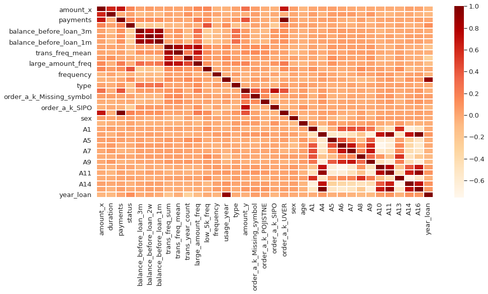
Linear Correlation among data
If two variables are highly correlated, keeping both variables may be redundant. Keeping only one will help reduce dimensionality withour much loss of information.
corr = data.corr()
plt.figure(figsize = (15, 7))
sns.heatmap(corr, cmap = 'OrRd', linewidths = 0.01)
Predictive Modeling
- baseline model:
- SVM
- other models:
- RandomForest
- AdaBoost
- GradientBoost
- XGBoost
features = data.columns.to_list()
features.remove('status')
SVM with linear kernel
from sklearn import svm
clf = svm.SVC(kernel = 'linear', C = 1, probability = True)
clf.fit(X_train, y_train)
clf.score(X_test, y_test) # accuracy
0.8947368421052632
# check the difference between target and prediction
# if result is not 0, it means target != prediction

diff = clf.predict(X_test) - y_test
diff[diff != 0]
68    -1
143   -1
555    1
19    -1
428   -1
237   -1
371   -1
435   -1
124   -1
340    1
128    1
230   -1
597    1
155   -1
301    1
132   -1
173    1
115   -1
291   -1
281   -1
408    1
383    1
493   -1
41    -1
Name: status, dtype: int64
# predict the probablity score for each class/category

clf.predict_proba(X_test)[:5]
array([[0.98444619, 0.01555381],
       [0.98370535, 0.01629465],
       [0.46087692, 0.53912308],
       [0.92077182, 0.07922818],
       [0.99238528, 0.00761472]])
# evaluation with sklearn's classification_report

from sklearn.metrics import classification_report
print(classification_report(y_test, clf.predict(X_test)))
              precision    recall  f1-score   support

           0       0.92      0.96      0.94       200
           1       0.60      0.43      0.50        28

    accuracy                           0.89       228
   macro avg       0.76      0.69      0.72       228
weighted avg       0.88      0.89      0.89       228
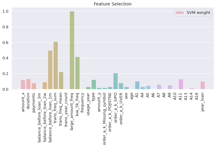
compare the SVM coeff
I visualized the SVM coefficient of each input feature by calculating the square and dividing by the maximum value to find the ratio. Larger coeff ratio indicates this feature has a greater impact
# process the svm weights by square
svm_weights = (clf.coef_ ** 2).sum(axis = 0)
svm_weights /= svm_weights.max() # indicates how large is the svm coeff of each feature

plt.figure(figsize = (12, 5))
sns.barplot(features, svm_weights, label = 'SVM weight', alpha = 0.6)

plt.title("Feature Selection")
plt.xticks(rotation = 90)
plt.axis('tight')
plt.legend(loc = 'upper right')
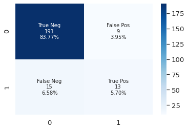
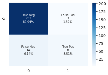
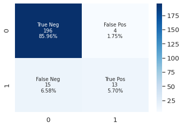
visualize the confusion matrix
Confusion Matrix can show the ground truth label vs prediction results. Therefore, we can figure out the model’s performance. For example, a false positive is the model predict a negative sample to positive, in our case is true label should be 0 but the prediction is 1. In our scenario, we should try to reduce the false negative.
from sklearn.metrics import confusion_matrix

def plot_cf_matrix(y_test, y_pred):
    '''
    Plot the confusion matrix.
    INPUT:
      - y_test: ground truth label
      - y_pred: model's prediction
    '''
    cf_matrix = confusion_matrix(y_test, y_pred)
    group_names = ['True Neg', 'False Pos', 'False Neg', 'True Pos']
    group_counts = ['{0:0.0f}'.format(value) for value in
                    cf_matrix.flatten()]
    group_percentages = ['{0:.2%}'.format(value) for value in
                         cf_matrix.flatten() / np.sum(cf_matrix)]
    labels = [f'{v1}\n{v2}\n{v3}' for v1, v2, v3 in
              zip(group_names,group_counts,group_percentages)]
    labels = np.asarray(labels).reshape(2, 2)

    sns.heatmap(cf_matrix, annot = labels, fmt = '', cmap = 'Blues')
y_pred = clf.predict(X_test)
plot_cf_matrix(y_test, y_pred)

SVM with normalized input
There are more than one scalers, I adopted StandardScaler in this case. If there are many outliers, better to choose other scalers such as robustscaler. In some cases, processing the data with normalization does not yield better results.
from sklearn.preprocessing import StandardScaler
# normalize the input data with standard scaler
sc = StandardScaler()
X = sc.fit_transform(X)
X_train, X_test, y_train, y_test = train_test_split(X, y, test_size = 1 / 3)
clf2 = svm.SVC(kernel = 'rbf', C = 10, probability = True)
clf2.fit(X_train, y_train)
clf2.score(X_test, y_test)
0.8947368421052632
print(classification_report(y_test, clf2.predict(X_test)))
              precision    recall  f1-score   support

           0       0.93      0.95      0.94       200
           1       0.59      0.46      0.52        28

    accuracy                           0.89       228
   macro avg       0.76      0.71      0.73       228
weighted avg       0.89      0.89      0.89       228
y_pred = clf2.predict(X_test)
plot_cf_matrix(y_test, y_pred)
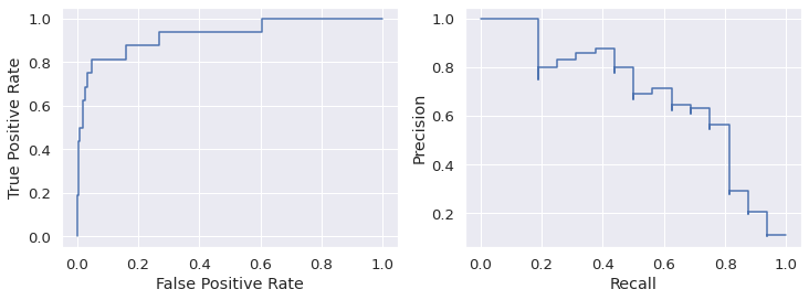
visualize the ROC curve and precision-recall curve
The roc curve requires either the probabilities or the non-thresholded decision values from the estimator.
from sklearn.metrics import precision_recall_curve, PrecisionRecallDisplay, roc_curve, RocCurveDisplay

y_score = clf2.decision_function(X_test)

fpr, tpr, _ = roc_curve(y_test, y_score, pos_label=clf2.classes_[1])
roc_display = RocCurveDisplay(fpr = fpr, tpr = tpr)

prec, recall, _ = precision_recall_curve(y_test, y_score,
                                         pos_label=clf2.classes_[1])
pr_display = PrecisionRecallDisplay(precision=prec, recall=recall)

fig, (ax1, ax2) = plt.subplots(1, 2, figsize=(12, 4))

roc_display.plot(ax = ax1)
pr_display.plot(ax = ax2)
Optimize the hyper-parameters of SVM with GridSearch
One headache in machine learning area is the hyper-parameter tuning. With grid search, this step is much easier. We can define all the hyper-parameters choices in the dictionary and it will run all and find out the best one.
from sklearn.model_selection import GridSearchCV
svc = svm.SVC()

param_grid = [{'C':[0.1,1,10], 'kernel':['linear']},
             {'C':[0.1,1,10], 'gamma':[0.001,0.01],'kernel':['rbf']}]

scoring = 'accuracy'
clfs = GridSearchCV(svc, param_grid, scoring = scoring, cv=10)
clfs.fit(X_train,y_train)
GridSearchCV(cv=10, estimator=SVC(),
             param_grid=[{'C': [0.1, 1, 10], 'kernel': ['linear']},
                         {'C': [0.1, 1, 10], 'gamma': [0.001, 0.01],
                          'kernel': ['rbf']}],
             scoring='accuracy')
print(clfs.best_estimator_)
SVC(C=0.1, kernel='linear')
from sklearn.metrics import classification_report

print(classification_report(y_test, clfs.best_estimator_.predict(X_test)))
              precision    recall  f1-score   support

           0       0.97      0.98      0.97       212
           1       0.64      0.56      0.60        16

    accuracy                           0.95       228
   macro avg       0.81      0.77      0.79       228
weighted avg       0.94      0.95      0.95       228
y_pred = clfs.best_estimator_.predict(X_test)
plot_cf_matrix(y_test, y_pred)
Try other models
- RandomForest
- AdaBoost
- GradientBoost
- XGBoost
script to visualize the feature importance
def visualize_coeff(model, name, feature_col = features):
    '''
    Function to visualize the coeff importance of each model
    INPUT:
      - model: the model instance
      - name: name of the model to show on title
      - feature_col: a list of column names of all features, default value set to be a global list named features
    OUTPUT:
      None
    '''
    coeff = model.feature_importances_

    importance = pd.DataFrame({"feature": features, 'importance': coeff})
    importance.sort_values(by = 'importance', ascending = False, inplace = True)

    plt.figure(figsize = (12, 5))
    plt.xticks(rotation = 90)

    sns.barplot(x = 'feature', y = 'importance', data = importance).set_title('The feature coeff of %s' % name)
Random Forest
from sklearn.ensemble import RandomForestClassifier

rf = RandomForestClassifier(max_depth = 2, random_state = 10)
rf.fit(X_train, y_train)
rf.score(X_test, y_test)
0.9122807017543859
print(classification_report(y_test, rf.predict(X_test)))
              precision    recall  f1-score   support

           0       0.92      1.00      0.95       206
           1       0.75      0.14      0.23        22

    accuracy                           0.91       228
   macro avg       0.83      0.57      0.59       228
weighted avg       0.90      0.91      0.88       228
visualize_coeff(rf, 'RandomForestClassifier')
y_pred = rf.predict(X_test)
plot_cf_matrix(y_test, y_pred)
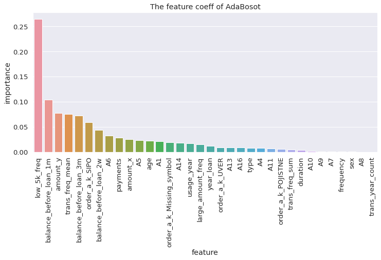
AdaBoost
from sklearn.ensemble import AdaBoostClassifier
adaboost = AdaBoostClassifier(n_estimators = 100)
adaboost.fit(X_train, y_train)
adaboost.score(X_test, y_test)
0.9254385964912281
print(classification_report(y_test, adaboost.predict(X_test)))
              precision    recall  f1-score   support

           0       0.97      0.95      0.96       212
           1       0.48      0.62      0.54        16

    accuracy                           0.93       228
   macro avg       0.72      0.79      0.75       228
weighted avg       0.94      0.93      0.93       228
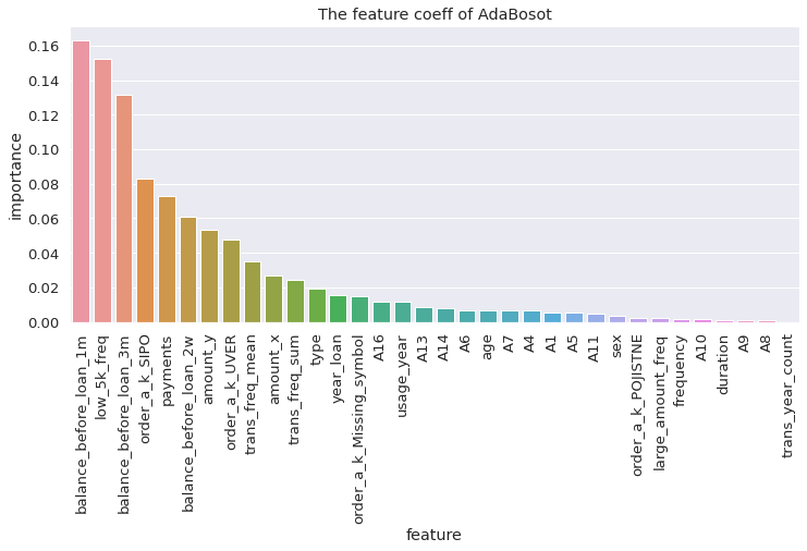
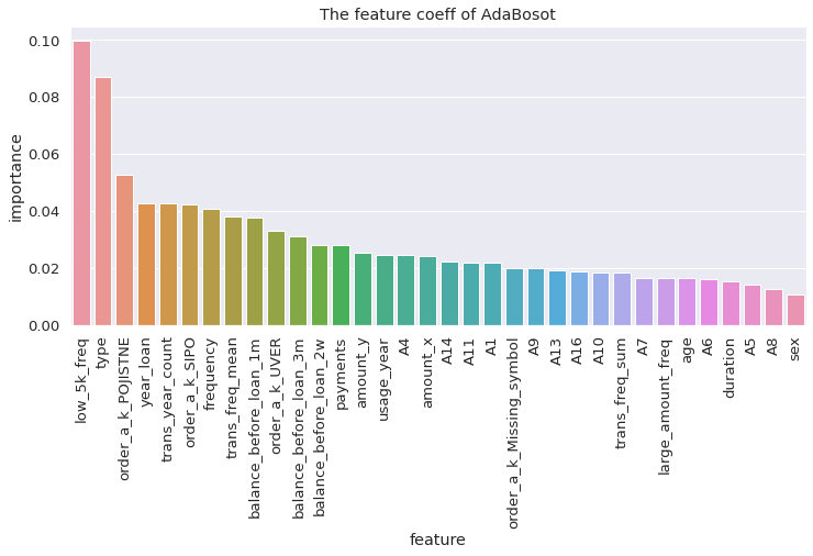
visualize_coeff(adaboost, 'AdaBoost')
Gradient Boosting
from sklearn.ensemble import GradientBoostingClassifier

dtc = GradientBoostingClassifier(n_estimators = 200, learning_rate = 0.1).fit(X_train, y_train)
dtc.score(X_test, y_test)
0.9122807017543859
print(classification_report(y_test, dtc.predict(X_test)))
              precision    recall  f1-score   support

           0       0.95      0.96      0.95       206
           1       0.55      0.50      0.52        22

    accuracy                           0.91       228
   macro avg       0.75      0.73      0.74       228
weighted avg       0.91      0.91      0.91       228
visualize_coeff(dtc, 'GradientBoostingClassifier')
XGBoost
from xgboost import XGBClassifier
xgb = XGBClassifier(colsample_bytree = 0.4603,
                    gamma            = 0.0468,
                    learning_rate    = 0.05,
                    max_depth        = 3,
                    min_child_weight = 1.7817,
                    n_estimators     = 2200,
                    reg_alpha        = 0.4640,
                    reg_lambda       = 0.8571,
                    subsample        = 0.5213,
                    silent           = 1,
                    random_state     = 7,
                    nthread          = -1)
xgb.fit(X_train, y_train)
xgb.score(X_test, y_test)
0.9166666666666666
print(classification_report(y_test, xgb.predict(X_test)))
              precision    recall  f1-score   support

           0       0.93      0.98      0.95       200
           1       0.76      0.46      0.58        28

    accuracy                           0.92       228
   macro avg       0.85      0.72      0.77       228
weighted avg       0.91      0.92      0.91       228
visualize_coeff(xgb, 'XGBoost')
y_pred = xgb.predict(X_test)
plot_cf_matrix(y_test, y_pred)
Conlusion
In this project, I fully clean the data and engineered features in order to make a dataset. I apply SVM as the baseline model, I try other models such as Random Forest, AdaBoost, GradientBoost, and XGBoost. I evaluate the performance and visualize the feature coeffs. In this use case, the most important evaluation metric should be the false negative and recall, because we may not approve the client’s loan application if the client has a high possibility to default on loans. Predicting the clients who may default on loans can help the bank apply the damage control policy. In addition, based on the data collected from the client’s transaction history and other information, bankers may have more practical standards when approving a client’s loan application.