New York Real Estate Analysis and Visualization with Seaborn and Folium
Introduction
In this notebook, I use the open source data of New York Real Estate transaction data. I first perform data cleaning and data exploration to understand the distribution of the data. Then I visualize the sales price distribution, compared with the median and mean sales price. The visualization results can help stakeholders understand better about the sales price distribution, especially when plotting on the map with Folium.
The tools and APIs used in this work include NumPy, Pandas, Seaborn, and Folium.
import numpy as np
import pandas as pd
import os
import warnings
import matplotlib.pyplot as plt
import seaborn as sns
import folium
from folium.plugins import MarkerCluster
%matplotlib inline
warnings.filterwarnings("ignore")
Pre-processing
Data pre-processing is the step to understand the data, and it is also an opportunity to verify the reliability of the data. It usually comes with the following steps:
- load the data
- check the length and shape of the data
- view head/tail lines of data
- remove useless data/columns
- check out the data type and NaN
- convert data types (such as string to datetime)
- handle missing values
Reading Data
Read the csv file with pandas function read_csv.
hsales = pd.read_csv('nyc-rolling-sales.csv')
check the shape
The shape of the dataframe indicates there are 22 columns and over 80k rows.
hsales.shape
(84548, 22)
Check the tail
See some real data samples with tail / head.
hsales.tail(10)
| Unnamed: 0 | BOROUGH | NEIGHBORHOOD | BUILDING CLASS CATEGORY | TAX CLASS AT PRESENT | BLOCK | LOT | EASE-MENT | BUILDING CLASS AT PRESENT | ADDRESS | ... | RESIDENTIAL UNITS | COMMERCIAL UNITS | TOTAL UNITS | LAND SQUARE FEET | GROSS SQUARE FEET | YEAR BUILT | TAX CLASS AT TIME OF SALE | BUILDING CLASS AT TIME OF SALE | SALE PRICE | SALE DATE | |
|---|---|---|---|---|---|---|---|---|---|---|---|---|---|---|---|---|---|---|---|---|---|
| 84538 | 8404 | 5 | WOODROW | 02 TWO FAMILY DWELLINGS | 1 | 7316 | 61 | B2 | 178 DARNELL LANE | ... | 2 | 0 | 2 | 3215 | 1300 | 1995 | 1 | B2 | - | 2017-06-30 00:00:00 | |
| 84539 | 8405 | 5 | WOODROW | 02 TWO FAMILY DWELLINGS | 1 | 7316 | 85 | B2 | 137 DARNELL LANE | ... | 2 | 0 | 2 | 3016 | 1300 | 1995 | 1 | B2 | - | 2016-12-30 00:00:00 | |
| 84540 | 8406 | 5 | WOODROW | 02 TWO FAMILY DWELLINGS | 1 | 7316 | 93 | B2 | 125 DARNELL LANE | ... | 2 | 0 | 2 | 3325 | 1300 | 1995 | 1 | B2 | 509000 | 2016-10-31 00:00:00 | |
| 84541 | 8407 | 5 | WOODROW | 02 TWO FAMILY DWELLINGS | 1 | 7317 | 126 | B2 | 112 ROBIN COURT | ... | 2 | 0 | 2 | 11088 | 2160 | 1994 | 1 | B2 | 648000 | 2016-12-07 00:00:00 | |
| 84542 | 8408 | 5 | WOODROW | 02 TWO FAMILY DWELLINGS | 1 | 7339 | 41 | B9 | 41 SONIA COURT | ... | 2 | 0 | 2 | 3020 | 1800 | 1997 | 1 | B9 | - | 2016-12-01 00:00:00 | |
| 84543 | 8409 | 5 | WOODROW | 02 TWO FAMILY DWELLINGS | 1 | 7349 | 34 | B9 | 37 QUAIL LANE | ... | 2 | 0 | 2 | 2400 | 2575 | 1998 | 1 | B9 | 450000 | 2016-11-28 00:00:00 | |
| 84544 | 8410 | 5 | WOODROW | 02 TWO FAMILY DWELLINGS | 1 | 7349 | 78 | B9 | 32 PHEASANT LANE | ... | 2 | 0 | 2 | 2498 | 2377 | 1998 | 1 | B9 | 550000 | 2017-04-21 00:00:00 | |
| 84545 | 8411 | 5 | WOODROW | 02 TWO FAMILY DWELLINGS | 1 | 7351 | 60 | B2 | 49 PITNEY AVENUE | ... | 2 | 0 | 2 | 4000 | 1496 | 1925 | 1 | B2 | 460000 | 2017-07-05 00:00:00 | |
| 84546 | 8412 | 5 | WOODROW | 22 STORE BUILDINGS | 4 | 7100 | 28 | K6 | 2730 ARTHUR KILL ROAD | ... | 0 | 7 | 7 | 208033 | 64117 | 2001 | 4 | K6 | 11693337 | 2016-12-21 00:00:00 | |
| 84547 | 8413 | 5 | WOODROW | 35 INDOOR PUBLIC AND CULTURAL FACILITIES | 4 | 7105 | 679 | P9 | 155 CLAY PIT ROAD | ... | 0 | 1 | 1 | 10796 | 2400 | 2006 | 4 | P9 | 69300 | 2016-10-27 00:00:00 |
10 rows × 22 columns
Remove unwanted columns
Drop columns with function drop and axis = 1.
hsales.drop(['Unnamed: 0','EASE-MENT'], axis = 1, inplace = True)
hsales.head(6)
| BOROUGH | NEIGHBORHOOD | BUILDING CLASS CATEGORY | TAX CLASS AT PRESENT | BLOCK | LOT | BUILDING CLASS AT PRESENT | ADDRESS | APARTMENT NUMBER | ZIP CODE | RESIDENTIAL UNITS | COMMERCIAL UNITS | TOTAL UNITS | LAND SQUARE FEET | GROSS SQUARE FEET | YEAR BUILT | TAX CLASS AT TIME OF SALE | BUILDING CLASS AT TIME OF SALE | SALE PRICE | SALE DATE | |
|---|---|---|---|---|---|---|---|---|---|---|---|---|---|---|---|---|---|---|---|---|
| 0 | 1 | ALPHABET CITY | 07 RENTALS - WALKUP APARTMENTS | 2A | 392 | 6 | C2 | 153 AVENUE B | 10009 | 5 | 0 | 5 | 1633 | 6440 | 1900 | 2 | C2 | 6625000 | 2017-07-19 00:00:00 | |
| 1 | 1 | ALPHABET CITY | 07 RENTALS - WALKUP APARTMENTS | 2 | 399 | 26 | C7 | 234 EAST 4TH STREET | 10009 | 28 | 3 | 31 | 4616 | 18690 | 1900 | 2 | C7 | - | 2016-12-14 00:00:00 | |
| 2 | 1 | ALPHABET CITY | 07 RENTALS - WALKUP APARTMENTS | 2 | 399 | 39 | C7 | 197 EAST 3RD STREET | 10009 | 16 | 1 | 17 | 2212 | 7803 | 1900 | 2 | C7 | - | 2016-12-09 00:00:00 | |
| 3 | 1 | ALPHABET CITY | 07 RENTALS - WALKUP APARTMENTS | 2B | 402 | 21 | C4 | 154 EAST 7TH STREET | 10009 | 10 | 0 | 10 | 2272 | 6794 | 1913 | 2 | C4 | 3936272 | 2016-09-23 00:00:00 | |
| 4 | 1 | ALPHABET CITY | 07 RENTALS - WALKUP APARTMENTS | 2A | 404 | 55 | C2 | 301 EAST 10TH STREET | 10009 | 6 | 0 | 6 | 2369 | 4615 | 1900 | 2 | C2 | 8000000 | 2016-11-17 00:00:00 | |
| 5 | 1 | ALPHABET CITY | 07 RENTALS - WALKUP APARTMENTS | 2 | 405 | 16 | C4 | 516 EAST 12TH STREET | 10009 | 20 | 0 | 20 | 2581 | 9730 | 1900 | 2 | C4 | - | 2017-07-20 00:00:00 |
print information
print the info of the dataframe to review the NaN and data type. It looks like empty records are not being treated as NA.
hsales.info()
<class 'pandas.core.frame.DataFrame'>
RangeIndex: 84548 entries, 0 to 84547
Data columns (total 20 columns):
BOROUGH                           84548 non-null int64
NEIGHBORHOOD                      84548 non-null object
BUILDING CLASS CATEGORY           84548 non-null object
TAX CLASS AT PRESENT              84548 non-null object
BLOCK                             84548 non-null int64
LOT                               84548 non-null int64
BUILDING CLASS AT PRESENT         84548 non-null object
ADDRESS                           84548 non-null object
APARTMENT NUMBER                  84548 non-null object
ZIP CODE                          84548 non-null int64
RESIDENTIAL UNITS                 84548 non-null int64
COMMERCIAL UNITS                  84548 non-null int64
TOTAL UNITS                       84548 non-null int64
LAND SQUARE FEET                  84548 non-null object
GROSS SQUARE FEET                 84548 non-null object
YEAR BUILT                        84548 non-null int64
TAX CLASS AT TIME OF SALE         84548 non-null int64
BUILDING CLASS AT TIME OF SALE    84548 non-null object
SALE PRICE                        84548 non-null object
SALE DATE                         84548 non-null object
dtypes: int64(9), object(11)
memory usage: 12.9+ MB
Converting data types
It looks like empty records are not being treated as NA. We convert columns to their appropriate data types to obtain NAs.
#First, let's check which columns should be categorical
print('Column name')
for col in hsales.columns:
    if hsales[col].dtype=='object':
        print(col, hsales[col].nunique())
Column name
NEIGHBORHOOD 254
BUILDING CLASS CATEGORY 47
TAX CLASS AT PRESENT 11
BUILDING CLASS AT PRESENT 167
ADDRESS 67563
APARTMENT NUMBER 3989
LAND SQUARE FEET 6062
GROSS SQUARE FEET 5691
BUILDING CLASS AT TIME OF SALE 166
SALE PRICE 10008
SALE DATE 364
# LAND SQUARE FEET,GROSS SQUARE FEET, SALE PRICE, BOROUGH should be numeric.
# SALE DATE datetime format.
# categorical: NEIGHBORHOOD, BUILDING CLASS CATEGORY, TAX CLASS AT PRESENT, BUILDING CLASS AT PRESENT,
# BUILDING CLASS AT TIME OF SALE, TAX CLASS AT TIME OF SALE,BOROUGH

numer = ['LAND SQUARE FEET','GROSS SQUARE FEET', 'SALE PRICE', 'BOROUGH']
for col in numer: # coerce for missing values
    hsales[col] = pd.to_numeric(hsales[col], errors = 'coerce')

categ = ['NEIGHBORHOOD', 'BUILDING CLASS CATEGORY', 'TAX CLASS AT PRESENT', 'BUILDING CLASS AT PRESENT', 'BUILDING CLASS AT TIME OF SALE', 'TAX CLASS AT TIME OF SALE']
for col in categ:
    hsales[col] = hsales[col].astype('category')

hsales['SALE DATE'] = pd.to_datetime(hsales['SALE DATE'], errors='coerce')
Our dataset is ready for checking missing values.
Check missing values
Find out which columns contain missing values, and calculate the percentage of the missing values in each column.
# find out which column has nan
hsales.isnull().any(axis = 0)
BOROUGH                           False
NEIGHBORHOOD                      False
BUILDING CLASS CATEGORY           False
TAX CLASS AT PRESENT              False
BLOCK                             False
LOT                               False
BUILDING CLASS AT PRESENT         False
ADDRESS                           False
APARTMENT NUMBER                  False
ZIP CODE                          False
RESIDENTIAL UNITS                 False
COMMERCIAL UNITS                  False
TOTAL UNITS                       False
LAND SQUARE FEET                   True
GROSS SQUARE FEET                  True
YEAR BUILT                        False
TAX CLASS AT TIME OF SALE         False
BUILDING CLASS AT TIME OF SALE    False
SALE PRICE                         True
SALE DATE                         False
dtype: bool
d = hsales.isnull().any(axis = 0).to_dict()
missing_col = [k for k in d if d[k] == True]
missing_col
['LAND SQUARE FEET', 'GROSS SQUARE FEET', 'SALE PRICE']
for col in missing_col:
    percentage = len(hsales[hsales[col].isna()]) / len(hsales)
    print('The percentage of missing values in the %s colume is %.2f%%.'%(col, percentage * 100))
The percentage of missing values in the LAND SQUARE FEET colume is 31.05%.
The percentage of missing values in the GROSS SQUARE FEET colume is 32.66%.
The percentage of missing values in the SALE PRICE colume is 17.22%.
missing = hsales.isnull()
missing.head(3)
| BOROUGH | NEIGHBORHOOD | BUILDING CLASS CATEGORY | TAX CLASS AT PRESENT | BLOCK | LOT | BUILDING CLASS AT PRESENT | ADDRESS | APARTMENT NUMBER | ZIP CODE | RESIDENTIAL UNITS | COMMERCIAL UNITS | TOTAL UNITS | LAND SQUARE FEET | GROSS SQUARE FEET | YEAR BUILT | TAX CLASS AT TIME OF SALE | BUILDING CLASS AT TIME OF SALE | SALE PRICE | SALE DATE | |
|---|---|---|---|---|---|---|---|---|---|---|---|---|---|---|---|---|---|---|---|---|
| 0 | False | False | False | False | False | False | False | False | False | False | False | False | False | False | False | False | False | False | False | False |
| 1 | False | False | False | False | False | False | False | False | False | False | False | False | False | False | False | False | False | False | True | False |
| 2 | False | False | False | False | False | False | False | False | False | False | False | False | False | False | False | False | False | False | True | False |
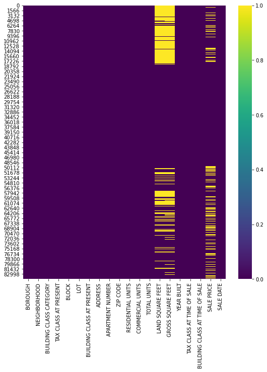
Around 30% of GROSS SF and LAND SF are missing. Furthermore, around 17% of SALE PRICE is also missing. Below graph indicates which parts of the table are missing values in yellow.
Data Analysis
The analysis in this notebook rely on data visualization.
Visualizing the missing values
We first visualize the missing values’ distribution.
plt.figure(figsize=(9, 10))
sns.heatmap(missing , cmap = 'viridis', cbar = True)
# let us check for outliers first
hsales[['LAND SQUARE FEET','GROSS SQUARE FEET']].describe()
| LAND SQUARE FEET | GROSS SQUARE FEET | |
|---|---|---|
| count | 5.829600e+04 | 5.693600e+04 |
| mean | 3.941676e+03 | 4.045707e+03 |
| std | 4.198397e+04 | 3.503249e+04 |
| min | 0.000000e+00 | 0.000000e+00 |
| 25% | 1.650000e+03 | 1.046750e+03 |
| 50% | 2.325000e+03 | 1.680000e+03 |
| 75% | 3.500000e+03 | 2.560000e+03 |
| max | 4.252327e+06 | 3.750565e+06 |
Visualizing the distribution that smaller than Q3
Plotting scatter, histogram, bar, and heatmap are some common approach to visualize the data distribution.
g = sns.JointGrid(x = 'LAND SQUARE FEET',
              y = 'GROSS SQUARE FEET',
              data = hsales[(hsales['LAND SQUARE FEET'] <= hsales['LAND SQUARE FEET'].quantile(.75))
                            & (hsales['GROSS SQUARE FEET']<= hsales['GROSS SQUARE FEET'].quantile(.75))],)

g.plot_joint(sns.scatterplot, s = 50, alpha = .8)
g.plot_marginals(sns.histplot, kde = True)
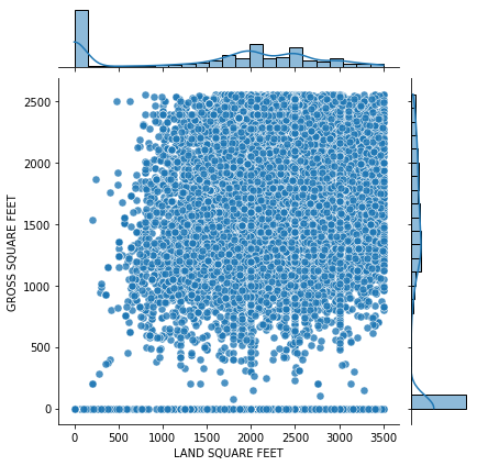
Check the correlation
The Pearson correlation coeff can tell us the linear relationship among variables. If the value is close to 1, the variables are positively correlated; if the value is close to -1, the variables are negatively correlated. 0 means there is no linear relationship.
The correlation check can help us to fill missing values.
hsales[(hsales['LAND SQUARE FEET'] <= 3500) & (hsales['GROSS SQUARE FEET'] <= 2560)][['LAND SQUARE FEET','GROSS SQUARE FEET']].corr()
| LAND SQUARE FEET | GROSS SQUARE FEET | |
|---|---|---|
| LAND SQUARE FEET | 1.000000 | 0.796219 |
| GROSS SQUARE FEET | 0.796219 | 1.000000 |
print(hsales[(hsales['LAND SQUARE FEET'].isnull()) & (hsales['GROSS SQUARE FEET'].notnull())].shape)
print(hsales[(hsales['LAND SQUARE FEET'].notnull()) & (hsales['GROSS SQUARE FEET'].isnull())].shape)
(6, 20)
(1366, 20)
There are 1366 rows that can be filled in with their approximate values. We fill GROSS SQUARE FEET when LAND SQUARE FEET is missing; and vice verse.
hsales['LAND SQUARE FEET'] = hsales['LAND SQUARE FEET'].mask((hsales['LAND SQUARE FEET'].isnull()) & (hsales['GROSS SQUARE FEET'].notnull()), hsales['GROSS SQUARE FEET'])
hsales['GROSS SQUARE FEET'] = hsales['GROSS SQUARE FEET'].mask((hsales['LAND SQUARE FEET'].notnull()) & (hsales['GROSS SQUARE FEET'].isnull()), hsales['LAND SQUARE FEET'])
# check duplicate values
print(sum(hsales.duplicated()))
hsales[hsales.duplicated(keep = False)].sort_values(['NEIGHBORHOOD', 'ADDRESS']).head(5)
# df.duplicated() automatically excludes duplicates, to keep duplicates in df we use keep=False
# in df.duplicated(df.columns) we can specify column names to look for duplicates only in those mentioned columns.
765
| BOROUGH | NEIGHBORHOOD | BUILDING CLASS CATEGORY | TAX CLASS AT PRESENT | BLOCK | LOT | BUILDING CLASS AT PRESENT | ADDRESS | APARTMENT NUMBER | ZIP CODE | RESIDENTIAL UNITS | COMMERCIAL UNITS | TOTAL UNITS | LAND SQUARE FEET | GROSS SQUARE FEET | YEAR BUILT | TAX CLASS AT TIME OF SALE | BUILDING CLASS AT TIME OF SALE | SALE PRICE | SALE DATE | |
|---|---|---|---|---|---|---|---|---|---|---|---|---|---|---|---|---|---|---|---|---|
| 76286 | 5 | ANNADALE | 02 TWO FAMILY DWELLINGS | 1 | 6350 | 7 | B2 | 106 BENNETT PLACE | 10312 | 2 | 0 | 2 | 8000.0 | 4208.0 | 1985 | 1 | B2 | NaN | 2017-06-27 | |
| 76287 | 5 | ANNADALE | 02 TWO FAMILY DWELLINGS | 1 | 6350 | 7 | B2 | 106 BENNETT PLACE | 10312 | 2 | 0 | 2 | 8000.0 | 4208.0 | 1985 | 1 | B2 | NaN | 2017-06-27 | |
| 76322 | 5 | ANNADALE | 05 TAX CLASS 1 VACANT LAND | 1B | 6459 | 28 | V0 | N/A HYLAN BOULEVARD | 0 | 0 | 0 | 0 | 6667.0 | 6667.0 | 0 | 1 | V0 | NaN | 2017-05-11 | |
| 76323 | 5 | ANNADALE | 05 TAX CLASS 1 VACANT LAND | 1B | 6459 | 28 | V0 | N/A HYLAN BOULEVARD | 0 | 0 | 0 | 0 | 6667.0 | 6667.0 | 0 | 1 | V0 | NaN | 2017-05-11 | |
| 76383 | 5 | ARDEN HEIGHTS | 01 ONE FAMILY DWELLINGS | 1 | 5741 | 93 | A5 | 266 ILYSSA WAY | 10312 | 1 | 0 | 1 | 500.0 | 1354.0 | 1996 | 1 | A5 | 320000.0 | 2017-06-06 |
Drop duplicates
Drop the duplicates to make our data cleaner.
hsales.drop_duplicates(inplace = True)
print(sum(hsales.duplicated()))
0
missing = hsales.isnull().sum() / len(hsales) * 100

print(pd.DataFrame([missing[missing > 0], pd.Series(hsales.isnull().sum()[hsales.isnull().sum() > 1000])],
                   index = ['percent missing', 'how many missing']))
                  LAND SQUARE FEET  GROSS SQUARE FEET  SALE PRICE
percent missing          31.091033          31.091033     16.9199
how many missing      26049.000000       26049.000000  14176.0000
print("The number of non-null prices for missing square feet observations:\n",
      ((hsales['LAND SQUARE FEET'].isnull()) & (hsales['SALE PRICE'].notnull())).sum())
The number of non-null prices for missing square feet observations:
 21154
print("non-overlapping observations that cannot be imputed:",
      ((hsales['LAND SQUARE FEET'].isnull()) & (hsales['SALE PRICE'].isnull())).sum())
non-overlapping observations that cannot be imputed: 4895
hsales[hsales['COMMERCIAL UNITS'] == 0].describe()
| BOROUGH | BLOCK | LOT | ZIP CODE | RESIDENTIAL UNITS | COMMERCIAL UNITS | TOTAL UNITS | LAND SQUARE FEET | GROSS SQUARE FEET | YEAR BUILT | SALE PRICE | |
|---|---|---|---|---|---|---|---|---|---|---|---|
| count | 78777.000000 | 78777.000000 | 78777.000000 | 78777.000000 | 78777.000000 | 78777.0 | 78777.000000 | 5.278000e+04 | 5.278000e+04 | 78777.000000 | 6.562900e+04 |
| mean | 3.004329 | 4273.781015 | 395.422420 | 10722.737068 | 1.691737 | 0.0 | 1.724133 | 3.140140e+03 | 2.714612e+03 | 1781.065451 | 9.952969e+05 |
| std | 1.298594 | 3589.241940 | 671.604654 | 1318.493961 | 9.838994 | 0.0 | 9.835016 | 2.929999e+04 | 2.791294e+04 | 551.024570 | 3.329268e+06 |
| min | 1.000000 | 1.000000 | 1.000000 | 0.000000 | 0.000000 | 0.0 | 0.000000 | 0.000000e+00 | 0.000000e+00 | 0.000000 | 0.000000e+00 |
| 25% | 2.000000 | 1330.000000 | 23.000000 | 10304.000000 | 0.000000 | 0.0 | 1.000000 | 1.600000e+03 | 9.750000e+02 | 1920.000000 | 2.400000e+05 |
| 50% | 3.000000 | 3340.000000 | 52.000000 | 11209.000000 | 1.000000 | 0.0 | 1.000000 | 2.295000e+03 | 1.600000e+03 | 1940.000000 | 5.294900e+05 |
| 75% | 4.000000 | 6361.000000 | 1003.000000 | 11357.000000 | 2.000000 | 0.0 | 2.000000 | 3.300000e+03 | 2.388000e+03 | 1967.000000 | 9.219560e+05 |
| max | 5.000000 | 16322.000000 | 9106.000000 | 11694.000000 | 889.000000 | 0.0 | 889.000000 | 4.252327e+06 | 4.252327e+06 | 2017.000000 | 3.450000e+08 |
# for visualization purposes, we replace borough numbering with their string names
hsales['BOROUGH'] = hsales['BOROUGH'].astype(str)
hsales['BOROUGH'] = hsales['BOROUGH'].str.replace("1", "Manhattan")
hsales['BOROUGH'] = hsales['BOROUGH'].str.replace("2", "Bronx")
hsales['BOROUGH'] = hsales['BOROUGH'].str.replace("3", "Brooklyn")
hsales['BOROUGH'] = hsales['BOROUGH'].str.replace("4", "Queens")
hsales['BOROUGH'] = hsales['BOROUGH'].str.replace("5", "Staten Island")
hsales.head(3)
| BOROUGH | NEIGHBORHOOD | BUILDING CLASS CATEGORY | TAX CLASS AT PRESENT | BLOCK | LOT | BUILDING CLASS AT PRESENT | ADDRESS | APARTMENT NUMBER | ZIP CODE | RESIDENTIAL UNITS | COMMERCIAL UNITS | TOTAL UNITS | LAND SQUARE FEET | GROSS SQUARE FEET | YEAR BUILT | TAX CLASS AT TIME OF SALE | BUILDING CLASS AT TIME OF SALE | SALE PRICE | SALE DATE | |
|---|---|---|---|---|---|---|---|---|---|---|---|---|---|---|---|---|---|---|---|---|
| 0 | Manhattan | ALPHABET CITY | 07 RENTALS - WALKUP APARTMENTS | 2A | 392 | 6 | C2 | 153 AVENUE B | 10009 | 5 | 0 | 5 | 1633.0 | 6440.0 | 1900 | 2 | C2 | 6625000.0 | 2017-07-19 | |
| 1 | Manhattan | ALPHABET CITY | 07 RENTALS - WALKUP APARTMENTS | 2 | 399 | 26 | C7 | 234 EAST 4TH STREET | 10009 | 28 | 3 | 31 | 4616.0 | 18690.0 | 1900 | 2 | C7 | NaN | 2016-12-14 | |
| 2 | Manhattan | ALPHABET CITY | 07 RENTALS - WALKUP APARTMENTS | 2 | 399 | 39 | C7 | 197 EAST 3RD STREET | 10009 | 16 | 1 | 17 | 2212.0 | 7803.0 | 1900 | 2 | C7 | NaN | 2016-12-09 |
hsales['BOROUGH'].value_counts()
Queens           26548
Brooklyn         23843
Manhattan        18102
Staten Island     8296
Bronx             6994
Name: BOROUGH, dtype: int64
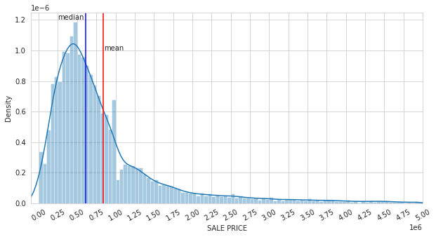
Visualize the distribution of Sale Price in(100, 5000000)
Visualize the distribution density of the sale price, compared with the median and mean value. Skewness can be figured by median/mean/mode relationship.
# house prices greater than 5 mln probably represents outliers.
import matplotlib.ticker as ticker
sns.set_style('whitegrid')
plt.figure(figsize = (10,5))
plotd = sns.distplot(hsales[(hsales['SALE PRICE'] > 100) & (hsales['SALE PRICE'] < 5000000 )]['SALE PRICE'],
                     kde = True, bins = 100)

tick_spacing = 250000 # set spacing for each tick
plotd.xaxis.set_major_locator(ticker.MultipleLocator(tick_spacing))
plotd.set_xlim([-100000, 5000000]) # do not show negative values
plt.xticks(rotation = 30) # rotate the xtick
plt.axvline(hsales[(hsales['SALE PRICE']>100) & (hsales['SALE PRICE'] < 5000000)]['SALE PRICE'].median(), c = 'b' )
plt.axvline(hsales[(hsales['SALE PRICE']>100) & (hsales['SALE PRICE'] < 5000000)]['SALE PRICE'].mean(), c = 'r')
plt.text(250000, 0.0000012, 'median')
plt.text(850000, 0.0000010, 'mean')
plt.show()
hsales['SALE PRICE'].describe()
count    6.960700e+04
mean     1.280703e+06
std      1.143036e+07
min      0.000000e+00
25%      2.300000e+05
50%      5.330000e+05
75%      9.500000e+05
max      2.210000e+09
Name: SALE PRICE, dtype: float64
dataset = hsales[(hsales['COMMERCIAL UNITS'] < 20)
                 & (hsales['TOTAL UNITS'] < 50)
                 & (hsales['SALE PRICE'] < 5000000)
                 & (hsales['SALE PRICE'] > 100000)
                 & (hsales['GROSS SQUARE FEET'] > 0)]#
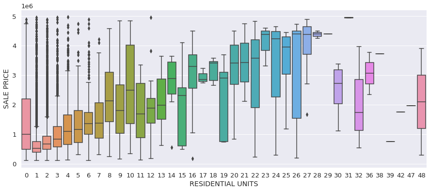
Visualize RESIDENTIAL UNITS vs SALE PRICE with boxplot
How sale price changes when residential units increase? Boxplot plots minimum, Q1, median, Q3, maximum, and outliers (greater than Q3 + 1.5 * IQR or smaller than Q1 - 1.5 * IQR).
plt.figure(figsize = (15, 6))
sns.set(font_scale = 1.2)
ax = sns.boxplot(x = "RESIDENTIAL UNITS", y = "SALE PRICE", data = dataset)
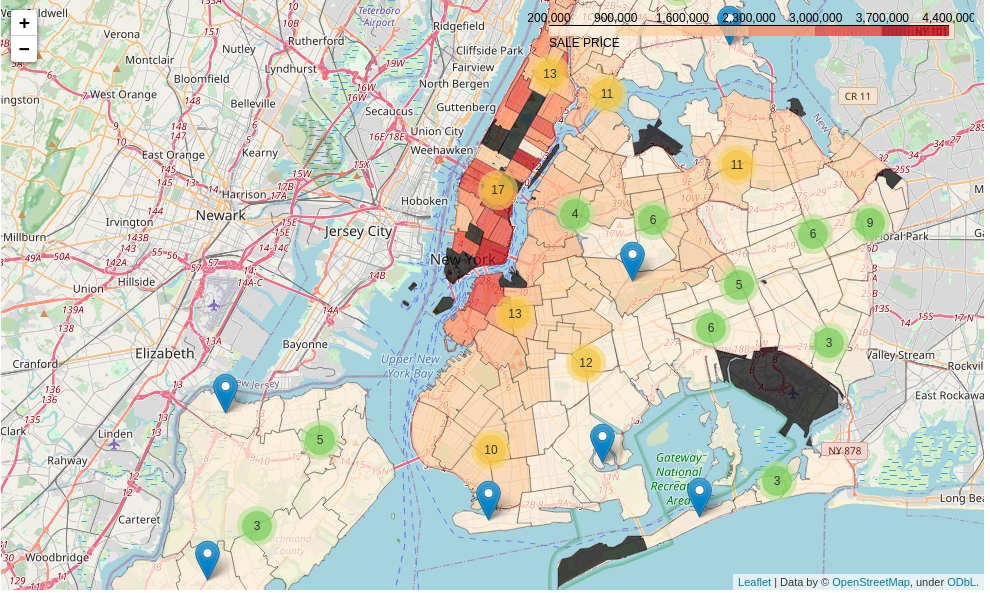
Visualize in map with Folium
Folium is a popular API used for visualizing geospatial data. I draw the marker clusters, otherwise the map would be overwhelmed by dense markers.
zipcodes = dataset[hsales["ZIP CODE"] > 0]
zipcodes['ZIP'] = zipcodes['ZIP CODE'].astype(str)
boroughs = zipcodes[['ZIP','BOROUGH']]
boroughs.drop_duplicates('ZIP', inplace = True)
us_zipcodes = pd.read_csv('uszipcodes_geodata.csv', delimiter = ',', dtype = str)
zipcodes_agg = pd.merge(zipcodes.groupby('ZIP').agg(np.mean), us_zipcodes, how = 'left', on = 'ZIP')
zipcodes_agg = pd.merge(zipcodes_agg, boroughs, how = 'left', on = 'ZIP')
zipcodes_agg.loc[116,'LAT'] = '40.6933'
zipcodes_agg.loc[116,'LNG'] = '-73.9925'
map = folium.Map(location = [40.693943, -73.985880], zoom_start = 11)
map.choropleth(geo_data = "nyc-zip-code-tabulation-areas-polygons.geojson",
             data = zipcodes_agg,
             columns = ['ZIP', 'SALE PRICE'],
             key_on = 'feature.properties.postalCode', # Variable in the geo_data GeoJSON file to bind the data to
             fill_color = 'OrRd', fill_opacity = 0.7, line_opacity = 0.3,
             legend_name = 'SALE PRICE')
marker_cluster = MarkerCluster().add_to(map) #  apply MarkerCluster into our map
for i in range(zipcodes_agg.shape[0]):
    location = [zipcodes_agg['LAT'][i],zipcodes_agg['LNG'][i]]
    tooltip = "Zipcode:{}<br> Borough: {}<br> Click for more".format(zipcodes_agg["ZIP"][i], zipcodes_agg['BOROUGH'][i])
    folium.Marker(location,
                  popup = """<i>Mean sales price: </i> <br> <b>${}</b> <br>
                  <i>mean total units: </i><b><br>{}</b><br>
                  <i>mean square feet: </i><b><br>{}</b><br>""".format(round(zipcodes_agg['SALE PRICE'][i],2),
                                                                       round(zipcodes_agg['TOTAL UNITS'][i],2),
                                                                       round(zipcodes_agg['GROSS SQUARE FEET'][i],2)),
                  tooltip = tooltip).add_to(marker_cluster)
map