Abstract of the project
Objective:
In this data challenge, I am going to work with 8 datasets from a bank (dataset was collected from year of 1999). Analyze the data and train the model to predict the customers that may default on loans.
Steps:
- Data pre-processing
- Load the data from .asc file into pd.DataFrame data structure.
- Transform the data into the ideal format and content.
- Rename and drop the columns if needed.
- Include some basic feature engineering for each table, such as encoding for categorical features and pivot.
- Analyze the data distribution by visualization.
- Feature Engineering and Dataset Preparation
- Merge some tables to create new features that may relate to the prediction.
- Merge all the tables together to feed to the model. Only in int and float type. Drop or fill the columns with null values.
- Conduct feature selection.
- Baseline model
- Begin with Linear SVM.
- Evaluation
- Visualize the coeff of features.
- Tune hyper-parameters for SVM.
- Try other models
- Random Forest
- AdaBoost
- Gradient Boosting
- XGBoost
- Concolusion
Note: This blog is part 2 of the whole project, only contains the feature engineering and dataset preparation. Please refer to the rest blogs for the following parts.
import pandas as pd
import numpy as np

import matplotlib.pyplot as plt
import seaborn as sns
sns.set(font_scale = 1.2)
%matplotlib inline
Feature Engineering and Dataset Preparation
Merge loan, account, and transaction tables.
- merge loan and account tables on acount_id
- merge with transaction table with account_id
With the merge function, we can define the key to be merged on, and the way to merge(inner, left, right, outer), we can customize the suffixes of the merged table if there are columns with same name in both tables.
loan_account = pd.merge(loan,
                        account,
                        how = 'left',
                        on = 'account_id',
                        suffixes = ('_loan','_acc'))
loan_account.head()
|
loan_id |
account_id |
date |
amount |
duration |
payments |
status |
district_id |
frequency |
usage_year |
| 0 |
5314 |
1787 |
1993-07-05 |
96396 |
12 |
8033.0 |
1 |
30 |
1 |
6 |
| 1 |
5316 |
1801 |
1993-07-11 |
165960 |
36 |
4610.0 |
0 |
46 |
2 |
6 |
| 2 |
6863 |
9188 |
1993-07-28 |
127080 |
60 |
2118.0 |
0 |
45 |
2 |
6 |
| 3 |
5325 |
1843 |
1993-08-03 |
105804 |
36 |
2939.0 |
0 |
12 |
2 |
6 |
| 4 |
7240 |
11013 |
1993-09-06 |
274740 |
60 |
4579.0 |
0 |
1 |
1 |
6 |
loan_account_trans = pd.merge(loan_account,
                              trans,
                              how = 'left',
                              on = 'account_id',
                              suffixes = ('_loan','_trans')
                             )
# display into two seperate parts just for the tight layout of the blog
display(loan_account_trans.iloc[:2, :11])
display(loan_account_trans.iloc[:2, 11:])
|
loan_id |
account_id |
date |
amount_loan |
duration |
payments |
status |
district_id |
frequency |
usage_year |
trans_id |
| 0 |
5314 |
1787 |
1993-07-05 |
96396 |
12 |
8033.0 |
1 |
30 |
1 |
6 |
523621 |
| 1 |
5314 |
1787 |
1993-07-05 |
96396 |
12 |
8033.0 |
1 |
30 |
1 |
6 |
524054 |
|
trans_date |
type |
operation |
amount_trans |
balance |
k_symbol |
bank |
account |
trans_type |
large_amount |
| 0 |
1993-03-22 |
PRIJEM |
VKLAD |
1100.0 |
1100.0 |
missing |
NaN |
NaN |
1.0 |
1 |
| 1 |
1993-04-21 |
PRIJEM |
VKLAD |
9900.0 |
11000.0 |
missing |
NaN |
NaN |
1.0 |
3 |
Calculate the date difference between loan and transaction
I use the date - transaction date to obtain the date difference between the loan grant date and the transaction date. Filters the records of transactions before loan approval to investigate clients’ financial situation and habbits. This also meets the actual needs: we need to analyze the past transactions to verify whether the client’s loan application can be approved.
- loan_trans_diff:
- greater than 0: indicates the transactions before the loan approval
- less than 0: indicates the transactions after the loan approval
loan_account_trans['loan_trans_diff'] = ((loan_account_trans['date'] - loan_account_trans['trans_date']) / np.timedelta64(1, 'D')).astype(int)
loan_account_trans = loan_account_trans[loan_account_trans['loan_trans_diff'] >= 0]
display(loan_account_trans.iloc[:2, :11])
display(loan_account_trans.iloc[:2, 11:])
|
loan_id |
account_id |
date |
amount_loan |
duration |
payments |
status |
district_id |
frequency |
usage_year |
trans_id |
| 0 |
5314 |
1787 |
1993-07-05 |
96396 |
12 |
8033.0 |
1 |
30 |
1 |
6 |
523621 |
| 1 |
5314 |
1787 |
1993-07-05 |
96396 |
12 |
8033.0 |
1 |
30 |
1 |
6 |
524054 |
|
trans_date |
type |
operation |
amount_trans |
balance |
k_symbol |
bank |
account |
trans_type |
large_amount |
loan_trans_diff |
| 0 |
1993-03-22 |
PRIJEM |
VKLAD |
1100.0 |
1100.0 |
missing |
NaN |
NaN |
1.0 |
1 |
105 |
| 1 |
1993-04-21 |
PRIJEM |
VKLAD |
9900.0 |
11000.0 |
missing |
NaN |
NaN |
1.0 |
3 |
75 |
Average transaction amount over the past period of time: 2 weeks, 1 month, and 3 months before loan date
What was the average transaction amount over the past period of time? Using groupby and aggregation can help us extract this information. The previous average transaction information can obtain the effective characteristics of the customer’s transaction habits. Therefore, these data can be used to determine whether the customer will default on repayment, and then the bank can consider approving or rejecting the loan application.
two_week = loan_account_trans[loan_account_trans['loan_trans_diff'] <= 14]
two_week = two_week.groupby(['loan_id'], as_index = None).mean()
two_week['balance_before_loan_2w'] = two_week['balance']
two_week = two_week.loc[:, ['loan_id', 'balance_before_loan_2w']]
display(two_week.head(5))
|
loan_id |
balance_before_loan_2w |
| 0 |
4959 |
25996.825 |
| 1 |
4962 |
35169.220 |
| 2 |
4967 |
31329.250 |
| 3 |
4968 |
32703.700 |
| 4 |
4973 |
24468.850 |
one_month = loan_account_trans[loan_account_trans['loan_trans_diff'] <= 30]
one_month = one_month.groupby(['loan_id'],as_index = None).mean()
one_month['balance_before_loan_1m'] = one_month['balance']
one_month = one_month.loc[:,['loan_id','balance_before_loan_1m']]
display(one_month.head(5))
|
loan_id |
balance_before_loan_1m |
| 0 |
4959 |
29349.755556 |
| 1 |
4961 |
14062.416667 |
| 2 |
4962 |
60769.460000 |
| 3 |
4967 |
33760.620000 |
| 4 |
4968 |
31890.450000 |
three_month = loan_account_trans[loan_account_trans['loan_trans_diff'] <= 90]
three_month = three_month.groupby(['loan_id'],as_index = None).mean()
three_month['balance_before_loan_3m'] = three_month['balance']
three_month = three_month.loc[:,['loan_id','balance_before_loan_3m']]
display(three_month.head(5))
|
loan_id |
balance_before_loan_3m |
| 0 |
4959 |
29830.005000 |
| 1 |
4961 |
15123.228571 |
| 2 |
4962 |
67547.706897 |
| 3 |
4967 |
20759.711111 |
| 4 |
4968 |
26212.342308 |
Transaction frequence
before = loan_account_trans
before['trans_year'] = before['trans_date'].dt.year # extract the year from datetime column
before.head(2)
|
loan_id |
account_id |
date |
amount_loan |
duration |
payments |
status |
district_id |
frequency |
usage_year |
... |
operation |
amount_trans |
balance |
k_symbol |
bank |
account |
trans_type |
large_amount |
loan_trans_diff |
trans_year |
| 0 |
5314 |
1787 |
1993-07-05 |
96396 |
12 |
8033.0 |
1 |
30 |
1 |
6 |
... |
VKLAD |
1100.0 |
1100.0 |
missing |
NaN |
NaN |
1.0 |
1 |
105 |
1993 |
| 1 |
5314 |
1787 |
1993-07-05 |
96396 |
12 |
8033.0 |
1 |
30 |
1 |
6 |
... |
VKLAD |
9900.0 |
11000.0 |
missing |
NaN |
NaN |
1.0 |
3 |
75 |
1993 |
2 rows × 23 columns
groupby loan id and the year of transaction date
trans_freq = before.loc[:, ['loan_id','trans_year','balance']].groupby(['loan_id','trans_year']).count()
trans_freq.rename(columns={'balance':'trans_freq'}, inplace = True)
trans_freq.head()
|
|
trans_freq |
| loan_id |
trans_year |
|
| 4959 |
1993 |
54 |
| 1994 |
1 |
| 4961 |
1995 |
54 |
| 1996 |
26 |
| 4962 |
1996 |
46 |
f = {'trans_freq': ['sum', 'mean'],
     'trans_year': ['count']}

trans_freq = trans_freq.reset_index().groupby('loan_id').agg(f)
trans_freq.columns = [s1 + '_' + s2 for (s1,s2) in trans_freq.columns.to_list()]
trans_freq.reset_index(inplace = True)
Number of large amount transactions
We encoded the transaction amount by quantile. If the transaction amount greater than Q3, then it is encoded to 3.
large_amount = before[before['large_amount'] == 3]
large_amount_freq = large_amount.loc[:,['loan_id','large_amount']].groupby(['loan_id']).count()
large_amount_freq.rename(columns = {'large_amount': 'large_amount_freq'}, inplace = True)
display(large_amount_freq.head())
|
large_amount_freq |
| loan_id |
|
| 4959 |
24 |
| 4961 |
26 |
| 4962 |
83 |
| 4967 |
32 |
| 4968 |
16 |
Number of transactions when balance lower than 5k
low_5k = before[before['balance'] <= 5000]
low_5k_freq = low_5k.loc[:,['loan_id', 'balance']].groupby(['loan_id']).count()
low_5k_freq.rename(columns = {'balance': 'low_5k_freq'},inplace = True)
display(low_5k_freq.head())
|
low_5k_freq |
| loan_id |
|
| 4959 |
1 |
| 4961 |
10 |
| 4962 |
1 |
| 4967 |
3 |
| 4973 |
1 |
Combine engineered features (transaction habbits)
loan_info = loan.merge(three_month,
                       how = 'left',
                       on = 'loan_id')

loan_info = loan_info.merge(two_week,
                            how = 'left',
                            on = 'loan_id')

loan_info = loan_info.merge(one_month,
                            how = 'left',
                            on = 'loan_id')

loan_info = loan_info.merge(trans_freq,
                            how = 'left',
                            on = 'loan_id')

loan_info = loan_info.merge(large_amount_freq,
                            how = 'left',
                            on = 'loan_id')

loan_info = loan_info.merge(low_5k_freq,
                            how = 'left',
                            on = 'loan_id')
loan_info.head()
|
loan_id |
account_id |
date |
amount |
duration |
payments |
status |
balance_before_loan_3m |
balance_before_loan_2w |
balance_before_loan_1m |
trans_freq_sum |
trans_freq_mean |
trans_year_count |
large_amount_freq |
low_5k_freq |
| 0 |
5314 |
1787 |
1993-07-05 |
96396 |
12 |
8033.0 |
1 |
15966.666667 |
NaN |
20100.000000 |
4 |
4.0 |
1 |
1.0 |
1.0 |
| 1 |
5316 |
1801 |
1993-07-11 |
165960 |
36 |
4610.0 |
0 |
56036.575862 |
36072.350000 |
33113.788889 |
37 |
37.0 |
1 |
14.0 |
2.0 |
| 2 |
6863 |
9188 |
1993-07-28 |
127080 |
60 |
2118.0 |
0 |
35160.929412 |
20272.800000 |
36233.066667 |
24 |
24.0 |
1 |
9.0 |
1.0 |
| 3 |
5325 |
1843 |
1993-08-03 |
105804 |
36 |
2939.0 |
0 |
46378.637500 |
34243.066667 |
42535.133333 |
25 |
25.0 |
1 |
13.0 |
1.0 |
| 4 |
7240 |
11013 |
1993-09-06 |
274740 |
60 |
4579.0 |
0 |
60804.547059 |
41127.900000 |
49872.757143 |
27 |
27.0 |
1 |
16.0 |
1.0 |
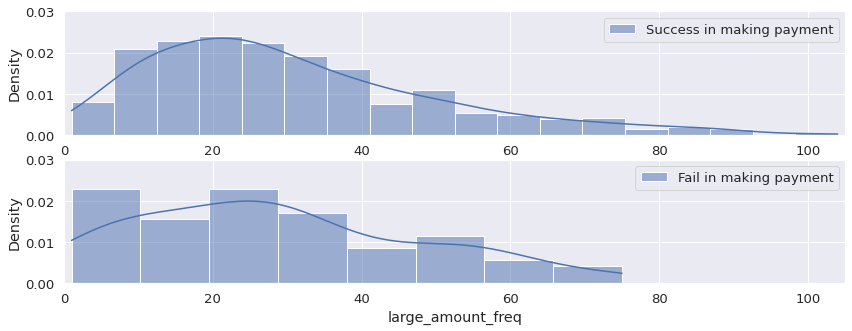
Compare two types of clients:
- status = 0: successfully make payments
- status = 1: fail to make payments
I observe their habits of large-amount transactions.
loan_info[loan_info['status'] == 0]['large_amount_freq'].describe()
count    605.000000
mean      30.737190
std       19.470525
min        1.000000
25%       16.000000
50%       26.000000
75%       41.000000
max      104.000000
Name: large_amount_freq, dtype: float64
loan_info[loan_info['status'] == 1]['large_amount_freq'].describe()
count    76.000000
mean     28.723684
std      19.039327
min       1.000000
25%      13.750000
50%      26.000000
75%      42.250000
max      75.000000
Name: large_amount_freq, dtype: float64
# making subplots to compare the payment habbits of these two types of clients
plt.figure(figsize = (14, 5))
plt.subplot(211)
sns.histplot(loan_info[loan_info['status'] == 0]['large_amount_freq'],
             stat = 'density', kde = True,
             label = 'Success in making payment')
plt.legend()
plt.ylim(0, 0.03)
plt.xlim(0, 105)

plt.subplot(212)
sns.histplot(loan_info[loan_info['status'] == 1]['large_amount_freq'],
             stat = 'density', kde = True,
             label = 'Fail in making payment')
plt.ylim(0, 0.03)
plt.xlim(0, 105)
plt.legend()
Merge all tables
data = pd.merge(loan_info,
                account,
                how = 'left',
                on = 'account_id'
               )
data = pd.merge(data,
                disp,
                how = 'left',
                on = 'account_id'
               )
data = pd.merge(data,
                card,
                how = 'left',
                on = 'disp_id'
               )
data = pd.merge(data,
                order,
                how = 'left',
                on = 'account_id'
               )
data = pd.merge(data,
                client,
                how = 'left',
                on = 'client_id'
               )
data = pd.merge(data,
                district,
                how = 'left',
                left_on = 'district_id_x',
                right_on = 'A1'
               )
display(data.iloc[:3, :10])
display(data.iloc[:3, 10: 21])
display(data.iloc[:3, 21: 30])
display(data.iloc[:3, 30:])
|
loan_id |
account_id |
date |
amount_x |
duration |
payments |
status |
balance_before_loan_3m |
balance_before_loan_2w |
balance_before_loan_1m |
| 0 |
5314 |
1787 |
1993-07-05 |
96396 |
12 |
8033.0 |
1 |
15966.666667 |
NaN |
20100.000000 |
| 1 |
5316 |
1801 |
1993-07-11 |
165960 |
36 |
4610.0 |
0 |
56036.575862 |
36072.35 |
33113.788889 |
| 2 |
6863 |
9188 |
1993-07-28 |
127080 |
60 |
2118.0 |
0 |
35160.929412 |
20272.80 |
36233.066667 |
|
trans_freq_sum |
trans_freq_mean |
trans_year_count |
large_amount_freq |
low_5k_freq |
district_id_x |
frequency |
usage_year |
disp_id |
client_id |
card_id |
| 0 |
4 |
4.0 |
1 |
1.0 |
1.0 |
30 |
1 |
6 |
2166 |
2166 |
NaN |
| 1 |
37 |
37.0 |
1 |
14.0 |
2.0 |
46 |
2 |
6 |
2181 |
2181 |
NaN |
| 2 |
24 |
24.0 |
1 |
9.0 |
1.0 |
45 |
2 |
6 |
11006 |
11314 |
NaN |
|
type |
issued |
amount_y |
order_a_k_LEASING |
order_a_k_Missing_symbol |
order_a_k_POJISTNE |
order_a_k_SIPO |
order_a_k_UVER |
birth_number |
| 0 |
NaN |
NaN |
8033.2 |
0.0 |
0.0 |
0.0 |
0.0 |
8033.2 |
475722 |
| 1 |
NaN |
NaN |
13152.0 |
0.0 |
3419.0 |
956.0 |
4167.0 |
4610.0 |
680722 |
| 2 |
NaN |
NaN |
10591.3 |
0.0 |
471.0 |
66.0 |
7936.0 |
2118.3 |
360602 |
|
district_id_y |
sex |
age |
A1 |
A4 |
A5 |
A6 |
A7 |
A8 |
A9 |
A10 |
A11 |
A12 |
A13 |
A14 |
A15 |
A16 |
| 0 |
30 |
1 |
52 |
30 |
94812 |
15 |
13 |
8 |
2 |
10 |
81.8 |
9650 |
3.38 |
3.67 |
100 |
2985 |
2804 |
| 1 |
46 |
0 |
31 |
46 |
112709 |
48 |
20 |
7 |
3 |
10 |
73.5 |
8369 |
1.79 |
2.31 |
117 |
2854 |
2618 |
| 2 |
45 |
0 |
63 |
45 |
77917 |
85 |
19 |
6 |
1 |
5 |
53.5 |
8390 |
2.28 |
2.89 |
132 |
2080 |
2122 |
data['year'] = data['date'].dt.year
data['year_loan'] = 1999 - (data['year']).astype(int)
Drop unnecessary columns
data.drop(['date','year', 'account_id', 'birth_number', 'card_id',
           'client_id', 'disp_id', 'district_id_x', 'district_id_y','issued',
           'loan_id', 'A12', 'A15'], axis = 1,  inplace = True)
Index(['amount_x', 'duration', 'payments', 'status', 'balance_before_loan_3m',
       'balance_before_loan_2w', 'balance_before_loan_1m', 'trans_freq_sum',
       'trans_freq_mean', 'trans_year_count', 'large_amount_freq',
       'low_5k_freq', 'frequency', 'usage_year', 'type', 'amount_y',
       'order_a_k_LEASING', 'order_a_k_Missing_symbol', 'order_a_k_POJISTNE',
       'order_a_k_SIPO', 'order_a_k_UVER', 'sex', 'age', 'A1', 'A4', 'A5',
       'A6', 'A7', 'A8', 'A9', 'A10', 'A11', 'A13', 'A14', 'A16', 'year_loan'],
      dtype='object')
data['type'].fillna(-1, inplace = True)
data.fillna(0, inplace = True)
data.info()
<class 'pandas.core.frame.DataFrame'>
Int64Index: 682 entries, 0 to 681
Data columns (total 36 columns):
amount_x                    682 non-null int64
duration                    682 non-null int64
payments                    682 non-null float64
status                      682 non-null int64
balance_before_loan_3m      682 non-null float64
balance_before_loan_2w      682 non-null float64
balance_before_loan_1m      682 non-null float64
trans_freq_sum              682 non-null int64
trans_freq_mean             682 non-null float64
trans_year_count            682 non-null int64
large_amount_freq           682 non-null float64
low_5k_freq                 682 non-null float64
frequency                   682 non-null int64
usage_year                  682 non-null int64
type                        682 non-null float64
amount_y                    682 non-null float64
order_a_k_LEASING           682 non-null float64
order_a_k_Missing_symbol    682 non-null float64
order_a_k_POJISTNE          682 non-null float64
order_a_k_SIPO              682 non-null float64
order_a_k_UVER              682 non-null float64
sex                         682 non-null int64
age                         682 non-null int64
A1                          682 non-null int64
A4                          682 non-null int64
A5                          682 non-null int64
A6                          682 non-null int64
A7                          682 non-null int64
A8                          682 non-null int64
A9                          682 non-null int64
A10                         682 non-null float64
A11                         682 non-null int64
A13                         682 non-null float64
A14                         682 non-null int64
A16                         682 non-null int64
year_loan                   682 non-null int64
dtypes: float64(16), int64(20)
memory usage: 197.1 KB
- the input are features
- the output should be the status: 0 / 1
I split train and test with a ratio of 2:1
from sklearn.model_selection import train_test_split

X = data.loc[:, data.columns != 'status']
y = data['status']

X_train, X_test, y_train, y_test = train_test_split(X, y, test_size = 1/3)
len(X_train), len(X_test)