Bank Loan Default Prediction with Pandas and Seaborn (Part 1)
Abstract of the project
Objective: In this data challenge, I am going to work with 8 datasets from a bank (dataset was collected from year of 1999). Analyze the data and train the model to predict the customers that may default on loans.
Steps for the whole project:
- Data pre-processing
- Load the data from .asc file into pd.DataFrame data structure.
- Transform the data into the ideal format and content.
- Rename and drop the columns if needed.
- Include some basic feature engineering for each table, such as encoding for categorical features and pivot.
- Analyze the data distribution by visualization.
- Feature Engineering and Dataset Preparation
- Merge some tables to create new features that may relate to the prediction.
- Merge all the tables together to feed to the model. Only in int and float type. Drop or fill the columns with null values.
- Conduct feature selection.
- Baseline model
- Begin with Linear SVM.
- Evaluation
- Visualize the coeff of features.
- Tune hyper-parameters for SVM.
- Try other models
- Random Forest
- AdaBoost
- Gradient Boosting
- XGBoost
- Concolusion
Note: This blog is part 1 of the whole project, only contains the data pre-processing for each table. Please refer to the rest blogs for the following parts.
import pandas as pd
import numpy as np
import matplotlib.pyplot as plt
import seaborn as sns
sns.set(font_scale = 1.2)
%matplotlib inline
Data pre-processing
- Load the data from 8 .asc files into pd.DataFrame data structure.
- Transform the data into the ideal format and content.
- Rename and drop the columns if needed.
- Include some basic feature engineering for each table, such as encoding for categorical features and pivot.
- Analyze the data distribution by visualization.
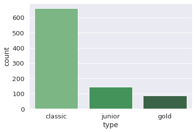
Credit Card Table
- Each record describes a credit card issued to an account.
- type: possible values are “junior”, “classic”, “gold”
card = pd.read_csv('card.asc', sep = ';')
display(card.head(2))
print(card.info())
| card_id | disp_id | type | issued | |
|---|---|---|---|---|
| 0 | 1005 | 9285 | classic | 931107 00:00:00 |
| 1 | 104 | 588 | classic | 940119 00:00:00 |
<class 'pandas.core.frame.DataFrame'>
RangeIndex: 892 entries, 0 to 891
Data columns (total 4 columns):
card_id    892 non-null int64
disp_id    892 non-null int64
type       892 non-null object
issued     892 non-null object
dtypes: int64(2), object(2)
memory usage: 28.0+ KB
None
sns.countplot(x = 'type', data = card, palette = 'Greens_d')
card['type'] = card['type'].map({'junior': 0, 'classic': 1, 'gold': 2})
card['issued'] = card['issued'].str.split(' ').str[0]
card.head(3)
| card_id | disp_id | type | issued | |
|---|---|---|---|---|
| 0 | 1005 | 9285 | 1 | 931107 |
| 1 | 104 | 588 | 1 | 940119 |
| 2 | 747 | 4915 | 1 | 940205 |
Disposition Table
- Each record relates together a client with an account i.e. this relation describes the rights of clients to operate accounts.
- type: Type of disposition (owner/user), Only owner can issue permanent orders and ask for a loan
disp = pd.read_csv('disp.asc', sep = ';')
display(disp.head(2))
print(disp.info(),'\n')
print(disp.type.value_counts())
| disp_id | client_id | account_id | type | |
|---|---|---|---|---|
| 0 | 1 | 1 | 1 | OWNER |
| 1 | 2 | 2 | 2 | OWNER |
<class 'pandas.core.frame.DataFrame'>
RangeIndex: 5369 entries, 0 to 5368
Data columns (total 4 columns):
disp_id       5369 non-null int64
client_id     5369 non-null int64
account_id    5369 non-null int64
type          5369 non-null object
dtypes: int64(3), object(1)
memory usage: 167.9+ KB
None

OWNER        4500
DISPONENT     869
Name: type, dtype: int64
disp = disp[disp['type'] == 'OWNER']
disp = disp.drop('type', axis = 1) # drop the type columns
print(disp.info())
disp.head(2)
<class 'pandas.core.frame.DataFrame'>
Int64Index: 4500 entries, 0 to 5368
Data columns (total 3 columns):
disp_id       4500 non-null int64
client_id     4500 non-null int64
account_id    4500 non-null int64
dtypes: int64(3)
memory usage: 140.6 KB
None
| disp_id | client_id | account_id | |
|---|---|---|---|
| 0 | 1 | 1 | 1 |
| 1 | 2 | 2 | 2 |
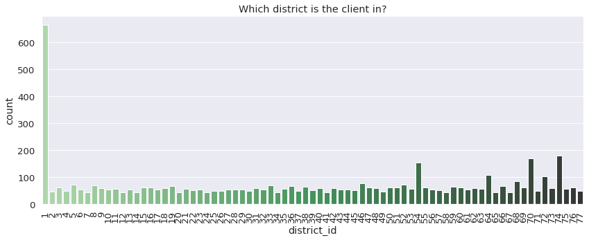
Client Table
- birth_number:
- the number is in the form YYMMDD for men
- the number is in the form YYMM+50DD for women
- where YYMMDD is the date of birth
- district_id: Address of the client
client = pd.read_csv('client.asc', sep = ';')
display(client.head(2))
print(client.info())
| client_id | birth_number | district_id | |
|---|---|---|---|
| 0 | 1 | 706213 | 18 |
| 1 | 2 | 450204 | 1 |
<class 'pandas.core.frame.DataFrame'>
RangeIndex: 5369 entries, 0 to 5368
Data columns (total 3 columns):
client_id       5369 non-null int64
birth_number    5369 non-null int64
district_id     5369 non-null int64
dtypes: int64(3)
memory usage: 126.0 KB
None
plt.figure(figsize = (14, 5))
plt.xticks(rotation = 90)
sns.countplot(x = 'district_id', data = client, palette = 'Greens_d').set_title('Which district is the client in?')
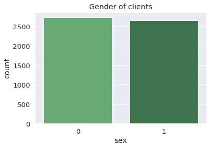
def birth_sex(column):
target = column['birth_number']
if target//100 % 100 > 50:
column['sex'] = 1 # female is 1
else:
column['sex'] = 0 # male is 0
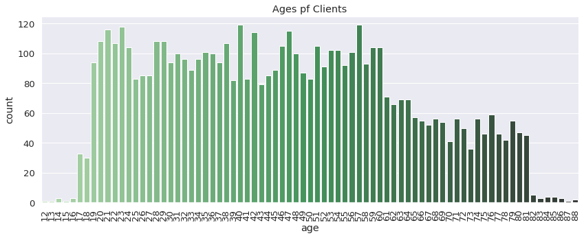
column['age'] = 99 - (target//10000)
return column
client = client.apply(birth_sex, axis = 1)
client.drop('birth_number', axis = 1)
client.head(2)
| client_id | birth_number | district_id | sex | age | |
|---|---|---|---|---|---|
| 0 | 1 | 706213 | 18 | 1 | 29 |
| 1 | 2 | 450204 | 1 | 0 | 54 |
sns.countplot(x = 'sex', data = client, palette = 'Greens_d').set_title('Gender of clients')
plt.figure(figsize = (14, 5))
plt.xticks(rotation = 90)
sns.countplot(x = 'age', data = client, palette = 'Greens_d').set_title('Ages pf Clients')
Account Table
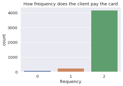
- frequency: Frequency of issuance of statements
- “POPLATEK MESICNE” stands for monthly issuance
- “POPLATEK TYDNE” stands for weekly issuance
- “POPLATEK PO OBRATU” stands for issuance after transaction
- date: Date of create of the account, in the form of YYMMDD
account = pd.read_csv('account.asc', sep = ';')
display(account.head(2))
print(account.info())
| account_id | district_id | frequency | date | |
|---|---|---|---|---|
| 0 | 576 | 55 | POPLATEK MESICNE | 930101 |
| 1 | 3818 | 74 | POPLATEK MESICNE | 930101 |
<class 'pandas.core.frame.DataFrame'>
RangeIndex: 4500 entries, 0 to 4499
Data columns (total 4 columns):
account_id     4500 non-null int64
district_id    4500 non-null int64
frequency      4500 non-null object
date           4500 non-null int64
dtypes: int64(3), object(1)
memory usage: 140.8+ KB
None
account['frequency'] = account['frequency'].map({"POPLATEK MESICNE": 2,
                                                 "POPLATEK TYDNE": 1,
                                                 "POPLATEK PO OBRATU": 0})

account['usage_year'] = 99 - account['date']//10000
account = account.drop('date', axis = 1)
account.head(3)
| account_id | district_id | frequency | usage_year | |
|---|---|---|---|---|
| 0 | 576 | 55 | 2 | 6 |
| 1 | 3818 | 74 | 2 | 6 |
| 2 | 704 | 55 | 2 | 6 |
sns.countplot(x = 'frequency', data = account).set_title('How frequency does the client pay the card')
sns.countplot(x = 'usage_year', data = account).set_title('How long has the client used the card')
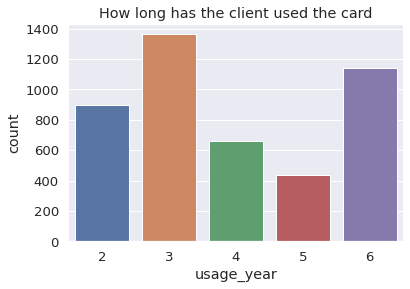
Table transaction
- trans_id: record identifier
- account_id: account, the transation deals with
- date: date of transaction in the form YYMMDD
- type: +/- transaction
- “PRIJEM” stands for credit
- “VYDAJ” stands for withdrawal
- operation: mode of transaction
- “VYBER KARTOU” credit card withdrawal
- “VKLAD” credit in cash
- “PREVOD Z UCTU” collection from another bank
- “VYBER” withdrawal in cash
- “PREVOD NA UCET” remittance to another bank
- amount
- balance: balance after transaction “POJISTNE” stands for insurrance payment
- “SLUZBY” stands for payment for statement
- “UROK” stands for interest credited
- “SANKC. UROK” sanction interest if negative balance
- “SIPO” stands for household
- “DUCHOD” stands for old-age pension
- “UVER” stands for loan payment
- k_symbol: characterization of the transaction
- bank: bank of the partner, each bank has unique two-letter code
- account: account of the partner
trans = pd.read_csv('trans.asc', sep = ';', low_memory = False)
display(trans.head())
print(trans.info()) # there are many NaNs in this table
| trans_id | account_id | date | type | operation | amount | balance | k_symbol | bank | account | |
|---|---|---|---|---|---|---|---|---|---|---|
| 0 | 695247 | 2378 | 930101 | PRIJEM | VKLAD | 700.0 | 700.0 | NaN | NaN | NaN |
| 1 | 171812 | 576 | 930101 | PRIJEM | VKLAD | 900.0 | 900.0 | NaN | NaN | NaN |
| 2 | 207264 | 704 | 930101 | PRIJEM | VKLAD | 1000.0 | 1000.0 | NaN | NaN | NaN |
| 3 | 1117247 | 3818 | 930101 | PRIJEM | VKLAD | 600.0 | 600.0 | NaN | NaN | NaN |
| 4 | 579373 | 1972 | 930102 | PRIJEM | VKLAD | 400.0 | 400.0 | NaN | NaN | NaN |
<class 'pandas.core.frame.DataFrame'>
RangeIndex: 1056320 entries, 0 to 1056319
Data columns (total 10 columns):
trans_id      1056320 non-null int64
account_id    1056320 non-null int64
date          1056320 non-null int64
type          1056320 non-null object
operation     873206 non-null object
amount        1056320 non-null float64
balance       1056320 non-null float64
k_symbol      574439 non-null object
bank          273508 non-null object
account       295389 non-null float64
dtypes: float64(3), int64(3), object(4)
memory usage: 80.6+ MB
None
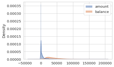
check the density distribution
sns.set_style('whitegrid')
sns.histplot(trans[['amount','balance']], stat = 'density', kde = True)
convert the data type, encode the trans_type
Categorical feautres has to be encoded. Since the data size is not large, we can directly use map to replace OrdinalEncoder.
trans['date'] = pd.to_datetime(trans['date'], format="%y%m%d")
trans.rename(columns = {'date':'trans_date'}, inplace = True)
trans['trans_type'] = trans['type'].map({'PRIJEM': 1, 'VYDAJ': -1})
trans.head()
| trans_id | account_id | trans_date | type | operation | amount | balance | k_symbol | bank | account | trans_type | |
|---|---|---|---|---|---|---|---|---|---|---|---|
| 0 | 695247 | 2378 | 1993-01-01 | PRIJEM | VKLAD | 700.0 | 700.0 | NaN | NaN | NaN | 1.0 |
| 1 | 171812 | 576 | 1993-01-01 | PRIJEM | VKLAD | 900.0 | 900.0 | NaN | NaN | NaN | 1.0 |
| 2 | 207264 | 704 | 1993-01-01 | PRIJEM | VKLAD | 1000.0 | 1000.0 | NaN | NaN | NaN | 1.0 |
| 3 | 1117247 | 3818 | 1993-01-01 | PRIJEM | VKLAD | 600.0 | 600.0 | NaN | NaN | NaN | 1.0 |
| 4 | 579373 | 1972 | 1993-01-02 | PRIJEM | VKLAD | 400.0 | 400.0 | NaN | NaN | NaN | 1.0 |
# check the operations for withdrawal
trans[trans['trans_type']==-1]['operation'].value_counts()
VYBER             418252
PREVOD NA UCET    208283
VYBER KARTOU        8036
Name: operation, dtype: int64
divide and encode the amount by quantile
To enrich the feature, we can divide the data by quantile and thereby encode into different levels according to the value.
trans[['amount','balance']].describe()
| amount | balance | |
|---|---|---|
| count | 1.056320e+06 | 1.056320e+06 |
| mean | 5.924146e+03 | 3.851833e+04 |
| std | 9.522735e+03 | 2.211787e+04 |
| min | 0.000000e+00 | -4.112570e+04 |
| 25% | 1.359000e+02 | 2.240250e+04 |
| 50% | 2.100000e+03 | 3.314340e+04 |
| 75% | 6.800000e+03 | 4.960362e+04 |
| max | 8.740000e+04 | 2.096370e+05 |
def amount_dist(column):
    '''
    Encoding a feature by comparing with quantile values
    '''
    if column['amount'] >= 6800: # quantile(.75) 75% distribution
        return 3
    elif column['amount'] >= 2100: # 50%
        return 2
    elif column['amount'] >= 136: # 25%
        return 1
    else:
        return 0
trans['large_amount'] = trans.apply(amount_dist, axis = 1)
display(trans.head(2))
| trans_id | account_id | trans_date | type | operation | amount | balance | k_symbol | bank | account | trans_type | large_amount | |
|---|---|---|---|---|---|---|---|---|---|---|---|---|
| 0 | 695247 | 2378 | 1993-01-01 | PRIJEM | VKLAD | 700.0 | 700.0 | NaN | NaN | NaN | 1.0 | 1 |
| 1 | 171812 | 576 | 1993-01-01 | PRIJEM | VKLAD | 900.0 | 900.0 | NaN | NaN | NaN | 1.0 | 1 |
# see an example
display(trans[trans['account_id'] == 576].head(8))
| trans_id | account_id | trans_date | type | operation | amount | balance | k_symbol | bank | account | trans_type | large_amount | |
|---|---|---|---|---|---|---|---|---|---|---|---|---|
| 1 | 171812 | 576 | 1993-01-01 | PRIJEM | VKLAD | 900.0 | 900.0 | NaN | NaN | NaN | 1.0 | 1 |
| 49 | 171813 | 576 | 1993-01-11 | PRIJEM | PREVOD Z UCTU | 6207.0 | 7107.0 | DUCHOD | YZ | 30300313.0 | 1.0 | 2 |
| 153 | 3549613 | 576 | 1993-01-31 | PRIJEM | NaN | 20.1 | 7127.1 | UROK | NaN | NaN | 1.0 | 0 |
| 308 | 171814 | 576 | 1993-02-11 | PRIJEM | PREVOD Z UCTU | 6207.0 | 13334.1 | DUCHOD | YZ | 30300313.0 | 1.0 | 2 |
| 508 | 3549614 | 576 | 1993-02-28 | PRIJEM | NaN | 29.6 | 13363.7 | UROK | NaN | NaN | 1.0 | 0 |
| 775 | 171815 | 576 | 1993-03-11 | PRIJEM | PREVOD Z UCTU | 6207.0 | 19570.7 | DUCHOD | YZ | 30300313.0 | 1.0 | 2 |
| 1146 | 3549615 | 576 | 1993-03-31 | PRIJEM | NaN | 29.6 | 19600.3 | UROK | NaN | NaN | 1.0 | 0 |
| 1517 | 171816 | 576 | 1993-04-11 | PRIJEM | PREVOD Z UCTU | 6207.0 | 25807.3 | DUCHOD | YZ | 30300313.0 | 1.0 | 2 |
pivot the operation and assign the amount to each operation
NaNs will not appear in the value_counts results.
print(trans['operation'].value_counts())
trans['operation'].fillna('missing operation', inplace = True)
trans['operation'].value_counts()
VYBER             434918
PREVOD NA UCET    208283
VKLAD             156743
PREVOD Z UCTU      65226
VYBER KARTOU        8036
Name: operation, dtype: int64


VYBER                434918
PREVOD NA UCET       208283
missing operation    183114
VKLAD                156743
PREVOD Z UCTU         65226
VYBER KARTOU           8036
Name: operation, dtype: int64
trans_op = trans.pivot(index = 'trans_id', columns = 'operation', values = 'amount')
trans_op.fillna(0, inplace = True)
trans_op.columns = ['a_missing operation','a_PREVOD NA UCET', 'a_PREVOD Z UCTU', 'a_VKLAD', 'a_VYBER',
       'a_VYBER KARTOU']
display(trans_op.head(2))
| a_missing operation | a_PREVOD NA UCET | a_PREVOD Z UCTU | a_VKLAD | a_VYBER | a_VYBER KARTOU | |
|---|---|---|---|---|---|---|
| trans_id | ||||||
| 1 | 0.0 | 0.0 | 1000.0 | 0.0 | 0.0 | 0.0 |
| 5 | 0.0 | 3679.0 | 0.0 | 0.0 | 0.0 | 0.0 |
pivot the k_symbol
NaNs are different from empty strings, so they need to be handled seperately. Before pivot the k_symbol, I handle the NaNs by fillna, and empty strings by using regex and loc.
trans['k_symbol'].fillna('missing', inplace = True)
trans['k_symbol'].value_counts()
missing        481881
UROK           183114
SLUZBY         155832
SIPO           118065
                53433
DUCHOD          30338
POJISTNE        18500
UVER            13580
SANKC. UROK      1577
Name: k_symbol, dtype: int64
trans['k_symbol'] = trans['k_symbol'].str.replace('\s+','', regex=True)
trans['k_symbol'].value_counts()
missing       481881
UROK          183114
SLUZBY        155832
SIPO          118065
               53433
DUCHOD         30338
POJISTNE       18500
UVER           13580
SANKC.UROK      1577
Name: k_symbol, dtype: int64
trans.loc[trans['k_symbol']=='', 'k_symbol'] = 'empty_symbol'
trans['k_symbol'].value_counts()
missing         481881
UROK            183114
SLUZBY          155832
SIPO            118065
empty_symbol     53433
DUCHOD           30338
POJISTNE         18500
UVER             13580
SANKC.UROK        1577
Name: k_symbol, dtype: int64
trans_ksymbol = trans.pivot(index = 'trans_id', columns = 'k_symbol', values = 'amount')
trans_ksymbol.columns = ['a_k_' + s for s in trans_ksymbol.columns.to_list()]
trans_ksymbol.fillna(0, inplace = True)
display(trans_ksymbol.head(2))
| a_k_DUCHOD | a_k_POJISTNE | a_k_SANKC.UROK | a_k_SIPO | a_k_SLUZBY | a_k_UROK | a_k_UVER | a_k_empty_symbol | a_k_missing | |
|---|---|---|---|---|---|---|---|---|---|
| trans_id | |||||||||
| 1 | 0.0 | 0.0 | 0.0 | 0.0 | 0.0 | 0.0 | 0.0 | 0.0 | 1000.0 |
| 5 | 0.0 | 0.0 | 0.0 | 0.0 | 0.0 | 0.0 | 0.0 | 0.0 | 3679.0 |
merge the trans with pivoted trans sub-tables
transdf = pd.merge(trans, trans_op, on = 'trans_id', how = 'inner')
transdf = pd.merge(transdf, trans_ksymbol, on = 'trans_id', how = 'inner')
transdf.drop(['k_symbol','operation','type','amount'] ,axis = 1, inplace = True)
display(transdf.iloc[:2, :12])
display(transdf.iloc[:2, 12:])
| trans_id | account_id | trans_date | balance | bank | account | trans_type | large_amount | a_missing operation | a_PREVOD NA UCET | a_PREVOD Z UCTU | a_VKLAD | |
|---|---|---|---|---|---|---|---|---|---|---|---|---|
| 0 | 695247 | 2378 | 1993-01-01 | 700.0 | NaN | NaN | 1.0 | 1 | 0.0 | 0.0 | 700.0 | 0.0 |
| 1 | 171812 | 576 | 1993-01-01 | 900.0 | NaN | NaN | 1.0 | 1 | 0.0 | 0.0 | 900.0 | 0.0 |
| a_VYBER | a_VYBER KARTOU | a_k_DUCHOD | a_k_POJISTNE | a_k_SANKC.UROK | a_k_SIPO | a_k_SLUZBY | a_k_UROK | a_k_UVER | a_k_empty_symbol | a_k_missing | |
|---|---|---|---|---|---|---|---|---|---|---|---|
| 0 | 0.0 | 0.0 | 0.0 | 0.0 | 0.0 | 0.0 | 0.0 | 0.0 | 0.0 | 0.0 | 700.0 |
| 1 | 0.0 | 0.0 | 0.0 | 0.0 | 0.0 | 0.0 | 0.0 | 0.0 | 0.0 | 0.0 | 900.0 |
Order Table
- K_symbol: type of the payment
- “POJISTNE” stands for insurrance payment
- “SIPO” stands for household payment
- “LEASING” stands for leasing
- “UVER” stands for loan payment
order = pd.read_csv('order.asc', sep = ';')
print(order.info())
order.head(2)
<class 'pandas.core.frame.DataFrame'>
RangeIndex: 6471 entries, 0 to 6470
Data columns (total 6 columns):
order_id      6471 non-null int64
account_id    6471 non-null int64
bank_to       6471 non-null object
account_to    6471 non-null int64
amount        6471 non-null float64
k_symbol      6471 non-null object
dtypes: float64(1), int64(3), object(2)
memory usage: 303.5+ KB
None
| order_id | account_id | bank_to | account_to | amount | k_symbol | |
|---|---|---|---|---|---|---|
| 0 | 29401 | 1 | YZ | 87144583 | 2452.0 | SIPO |
| 1 | 29402 | 2 | ST | 89597016 | 3372.7 | UVER |
handle empty rows
# replace the empty k_symbols
order['k_symbol'] = order['k_symbol'].str.replace(' ', 'Missing_symbol')
order['k_symbol'].value_counts()
SIPO              3502
Missing_symbol    1379
UVER               717
POJISTNE           532
LEASING            341
Name: k_symbol, dtype: int64
pivot the k_symbol and fill with amount
# using pivot to create a df by k_symbol and fill the value with amount
order_pivot = order.pivot(index = 'order_id', columns = 'k_symbol', values = 'amount')
order_pivot.columns = ['order_a_k_' + s for s in order_pivot.columns.to_list()]
order_pivot.fillna(0, inplace = True)
display(order_pivot.head(2))
| order_a_k_LEASING | order_a_k_Missing_symbol | order_a_k_POJISTNE | order_a_k_SIPO | order_a_k_UVER | |
|---|---|---|---|---|---|
| order_id | |||||
| 29401 | 0.0 | 0.0 | 0.0 | 2452.0 | 0.0 |
| 29402 | 0.0 | 0.0 | 0.0 | 0.0 | 3372.7 |
merge two df and drop unnecessary columns
# join the tables together
order = pd.merge(order, order_pivot, on = 'order_id', how = 'left')
order.drop(['order_id','bank_to','account_to','k_symbol'], axis = 1, inplace = True)
order.head(2)
| account_id | amount | order_a_k_LEASING | order_a_k_Missing_symbol | order_a_k_POJISTNE | order_a_k_SIPO | order_a_k_UVER | |
|---|---|---|---|---|---|---|---|
| 0 | 1 | 2452.0 | 0.0 | 0.0 | 0.0 | 2452.0 | 0.0 |
| 1 | 2 | 3372.7 | 0.0 | 0.0 | 0.0 | 0.0 | 3372.7 |
sum up each account’s amount by groupby aggregation
order = order.groupby('account_id').sum()
order.head(3)
| amount | order_a_k_LEASING | order_a_k_Missing_symbol | order_a_k_POJISTNE | order_a_k_SIPO | order_a_k_UVER | |
|---|---|---|---|---|---|---|
| account_id | ||||||
| 1 | 2452.0 | 0.0 | 0.0 | 0.0 | 2452.0 | 0.0 |
| 2 | 10638.7 | 0.0 | 0.0 | 0.0 | 7266.0 | 3372.7 |
| 3 | 5001.0 | 0.0 | 327.0 | 3539.0 | 1135.0 | 0.0 |
Loan Table
- status: status of paying off the loan
- ‘A’ stands for contract finished, no problems
- ‘B’ stands for contract finished, loan not payed
- ‘C’ stands for running contract, OK so far
- ‘D’ stands for running contract, client in debt
- payment: monthly payment
I am going to encode the status into 0 with success (A,C), and 1 with fail to pay (B,D)
loan = pd.read_csv('loan.asc', sep = ';')
loan.head()
| loan_id | account_id | date | amount | duration | payments | status | |
|---|---|---|---|---|---|---|---|
| 0 | 5314 | 1787 | 930705 | 96396 | 12 | 8033.0 | B |
| 1 | 5316 | 1801 | 930711 | 165960 | 36 | 4610.0 | A |
| 2 | 6863 | 9188 | 930728 | 127080 | 60 | 2118.0 | A |
| 3 | 5325 | 1843 | 930803 | 105804 | 36 | 2939.0 | A |
| 4 | 7240 | 11013 | 930906 | 274740 | 60 | 4579.0 | A |
check the status distribution
Class imbalance is not unexpected. There are some common ways to cope with class imbalance, such as sampling. If using deep learning models, then can also consider to use Focal Loss.
loan['status'].value_counts()
C    403
A    203
D     45
B     31
Name: status, dtype: int64
convert to datetime and encoding categorical feature
loan['date'] = pd.to_datetime(loan['date'], format="%y%m%d")
loan['status'] = loan.status.map({'A': 0, 'B': 1,'C': 0, 'D': 1})
loan.info()
<class 'pandas.core.frame.DataFrame'>
RangeIndex: 682 entries, 0 to 681
Data columns (total 7 columns):
loan_id       682 non-null int64
account_id    682 non-null int64
date          682 non-null datetime64[ns]
amount        682 non-null int64
duration      682 non-null int64
payments      682 non-null float64
status        682 non-null int64
dtypes: datetime64[ns](1), float64(1), int64(5)
memory usage: 37.4 KB
display(loan.head(3))
| loan_id | account_id | date | amount | duration | payments | status | |
|---|---|---|---|---|---|---|---|
| 0 | 5314 | 1787 | 1993-07-05 | 96396 | 12 | 8033.0 | 1 |
| 1 | 5316 | 1801 | 1993-07-11 | 165960 | 36 | 4610.0 | 0 |
| 2 | 6863 | 9188 | 1993-07-28 | 127080 | 60 | 2118.0 | 0 |
District Table
This table provides demographic data, such as the crime rate of each district. These demographic data can reflect the user’s background and financial status.
- A1 = district_id District code
- A2 District name
- A3 Region
- A4 no. Of inhabitants
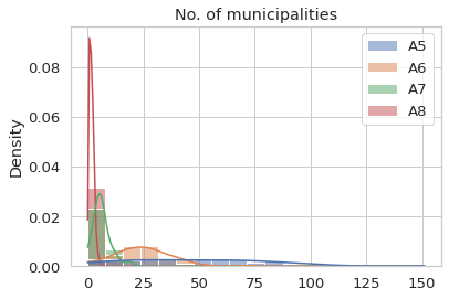
- A5 no. of municipalities with inhabitants < 499
- A6 no. of municipalities with inhabitants 500-1999
- A7 no. of municipalities with inhabitants 2000-9999
- A8 no. of municipalities with inhabitants >10000
- A9 no. of cities
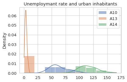
- A10 ratio of urban inhabitants
- A11 average salary
- A12 unemploymant rate ‘95
- A13 unemploymant rate ‘96
- A14 no. of enterpreneurs per 1000 inhabitants
- A15 no. of commited crimes ‘95
- A16 no. of commited crimes ‘96
district = pd.read_csv('district.asc', sep = ';')
district.drop(['A2','A3'], axis = 1, inplace = True)
district.head(3)
| A1 | A4 | A5 | A6 | A7 | A8 | A9 | A10 | A11 | A12 | A13 | A14 | A15 | A16 | |
|---|---|---|---|---|---|---|---|---|---|---|---|---|---|---|
| 0 | 1 | 1204953 | 0 | 0 | 0 | 1 | 1 | 100.0 | 12541 | 0.29 | 0.43 | 167 | 85677 | 99107 |
| 1 | 2 | 88884 | 80 | 26 | 6 | 2 | 5 | 46.7 | 8507 | 1.67 | 1.85 | 132 | 2159 | 2674 |
| 2 | 3 | 75232 | 55 | 26 | 4 | 1 | 5 | 41.7 | 8980 | 1.95 | 2.21 | 111 | 2824 | 2813 |
district.describe()
| A1 | A4 | A5 | A6 | A7 | A8 | A9 | A10 | A11 | A13 | A14 | A16 | |
|---|---|---|---|---|---|---|---|---|---|---|---|---|
| count | 77.000000 | 7.700000e+01 | 77.000000 | 77.000000 | 77.000000 | 77.000000 | 77.000000 | 77.000000 | 77.000000 | 77.000000 | 77.000000 | 77.000000 |
| mean | 39.000000 | 1.338849e+05 | 48.623377 | 24.324675 | 6.272727 | 1.727273 | 6.259740 | 63.035065 | 9031.675325 | 3.787013 | 116.129870 | 5030.831169 |
| std | 22.371857 | 1.369135e+05 | 32.741829 | 12.780991 | 4.015222 | 1.008338 | 2.435497 | 16.221727 | 790.202347 | 1.908480 | 16.608773 | 11270.796786 |
| min | 1.000000 | 4.282100e+04 | 0.000000 | 0.000000 | 0.000000 | 0.000000 | 1.000000 | 33.900000 | 8110.000000 | 0.430000 | 81.000000 | 888.000000 |
| 25% | 20.000000 | 8.585200e+04 | 22.000000 | 16.000000 | 4.000000 | 1.000000 | 5.000000 | 51.900000 | 8512.000000 | 2.310000 | 105.000000 | 2122.000000 |
| 50% | 39.000000 | 1.088710e+05 | 49.000000 | 25.000000 | 6.000000 | 2.000000 | 6.000000 | 59.800000 | 8814.000000 | 3.600000 | 113.000000 | 3040.000000 |
| 75% | 58.000000 | 1.390120e+05 | 71.000000 | 32.000000 | 8.000000 | 2.000000 | 8.000000 | 73.500000 | 9317.000000 | 4.790000 | 126.000000 | 4595.000000 |
| max | 77.000000 | 1.204953e+06 | 151.000000 | 70.000000 | 20.000000 | 5.000000 | 11.000000 | 100.000000 | 12541.000000 | 9.400000 | 167.000000 | 99107.000000 |
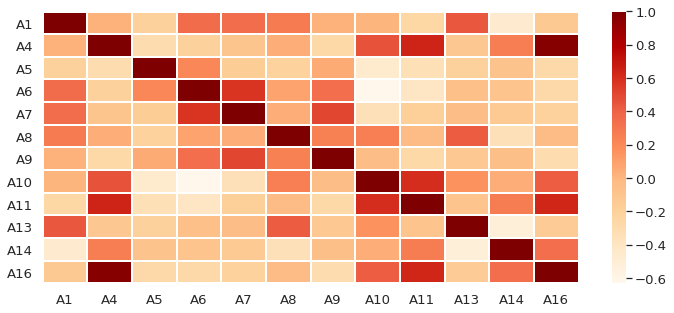
Check the pearson correlation of the district features
The Pearson correlation coeff can tell us the linear relationship among variables. If the value is close to 1, the variables are positively correlated; if the value is close to -1, the variables are negatively correlated. 0 means there is no linear relationship.
corr = district.corr()
plt.figure(figsize = (12, 5))
sns.heatmap(corr, cmap = 'OrRd', linewidths = 0.01)
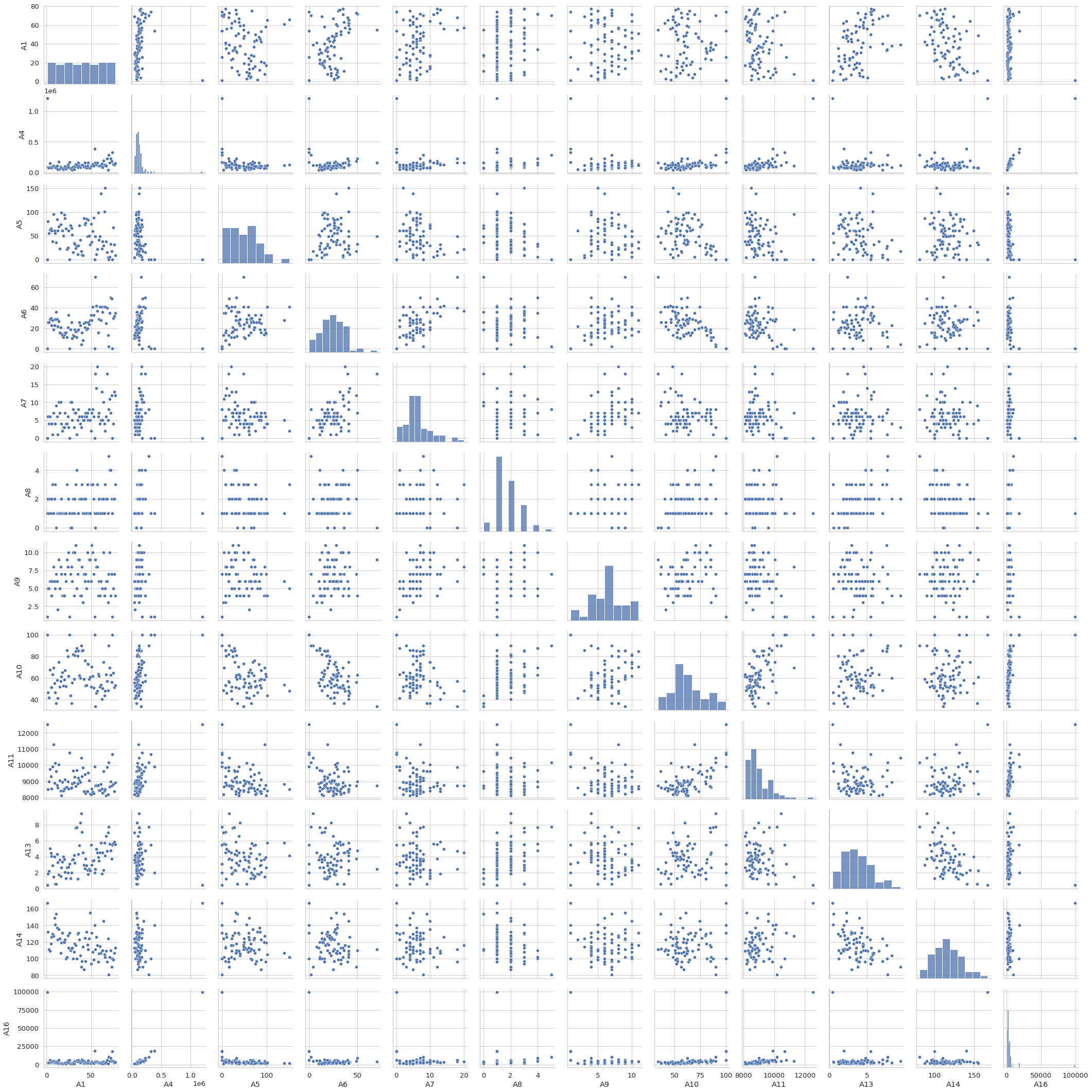
sns.pairplot(district, size = 2.5)
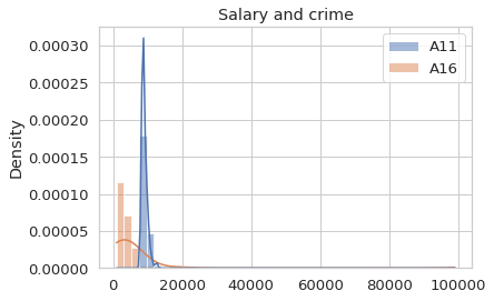
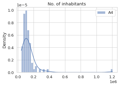
Visualize the density distribution of some demographic data
The visualization can help us to understand better of the data.
sns.histplot(district[['A4']], stat = 'density', kde = True).set_title('No. of inhabitants')
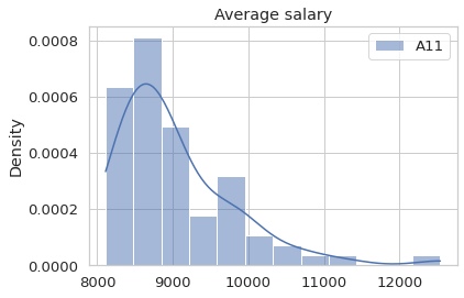
sns.histplot(district[['A11']], stat = 'density', kde = True).set_title('Average salary')
sns.histplot(district[['A5','A6','A7','A8']], stat = 'density', kde = True).set_title('No. of municipalities')
sns.histplot(district[['A10','A12','A13','A14']], stat = 'density', kde = True).set_title('Unemploymant rate and urban inhabitants')
sns.histplot(district[['A11','A16']], stat = 'density', kde = True).set_title('Salary and crime')